R E S E A R C H A R T I C L E
Open Access
Multi-GPU based on multicriteria optimization
for motion estimation system
Carlos Garcia
*, Guillermo Botella, Fermin Ayuso, Manuel Prieto and Francisco Tirado
Abstract
Graphics processor units (GPUs) offer high performance and power efficiency for a large number of data-parallel applications. Previous research has shown that a GPU-based version of a neuromorphic motion estimation algorithm can achieve a×32 speedup using these devices. However, the memory consumption creates a bottleneck due to the expansive tree of signal processing operations performed. In the present contribution, an improvement in memory reduction was carried out, which limited accelerator viability usage. An evolutionary algorithm was used to find the best configuration. It supposes a trade-off solution between consumption resources, parallel efficiency, and accuracy. A multilevel parallel scheme was exploited: grain level by means of multi-GPU systems, and a finer level by data parallelism. In order to achieve a more relevant analysis, some optical flow benchmarks were used to validate this study. Satisfactory results opened the chance of building an intelligent motion estimation system that auto-adapted according to real-time, resource consumption, and accuracy requirements.
Keywords: GPGPU, Motion estimation, Memory reduction technique, Multiobjective optimization
1 Introduction
Motion estimation and compensation are crucial for mul-timedia coding characterized by high memory require-ments and computation complexity. When considering MPEG processing, motion estimation is acknowledged as the most time-consuming [1], creating up to 90% of the total execution time [2,3]. Additionally, motion esti-mation has several applications regarding multimedia scope as segmentation, extraction of 3D structure, pat-tern tracking, filtering, compression, and de-blurring. Differently developed motion estimation models and algorithms can be classified into three main categories: matching domain approximations [4], energy models [5], and gradient models [6].
Block matching algorithms have the pros of robustness, low cost VLSI implementation (because of their regular parallel procedure), and low overhead (since they con-tain one vector per block). Nevertheless, there are many cons, since a block may contain several moving objects and fail for zoom, rotational motion, local deformation, and blocking artifact. In additional, they usually estimate
*Correspondence: [email protected]
Computer Architecture Deparment, Complutense University of Madrid, Madrid, Spain
the motion error by minimizing a metric, which does not release the true movement, etc. Energy models are probabilistic, delivering a population of solutions that do not indicate motion itself and are not usually used for multimedia purposes.
The gradient-based family can estimate vector motion of every single pixel, giving a dense representation of the processed frame. There are several examples of video compression using gradient based algorithm [7]. Recur-sive algorithms belonging to this family do not have to transmit motion information. Nevertheless, this algo-rithm family has the drawback of large motion vectors (severe motion), noisy images, and changes in illumina-tion. The present approach is based on a Multichannel Gradient Model (McGM) [8-10], a neuromorphic algo-rithm fitted to allow the construction of viable, highly robust, front-end processors for image recognition systems [11].
The increased computing capabilities of graphics pro-cessing units (GPUs) in recent years has increased their use as accelerators in many areas such as scientific sim-ulations, computer vision, bioinformatics, cryptography, and finance, among others. This increase is largely due to impressive performance rates. For example, one of the latest GPUs from Nvidia, the GTX 680, achieves
three petaflops in single precision with 1006 cores and also incorporates the newerKeplerarchitecture. Current trends seem to indicate that this capacity will grow even more with the incorporation of 22 and 28 nm technolo-gies. Recently, for example, AMD announced its Radeon 8000 Series, branded as Sea Island, and Intel is manu-facturing Knights Corner products. However, key points that dramatically affect performance rates include the effi-cient use of the memory hierarchy and the exploitation of parallelism capabilities.
The increased demand for information to be processed also plays a role, because the use of these devices as accel-erators is limited due to DDR memory restrictions. To solve this problem, research [12] has often proposed a data reuse alternative with the aim of minimizing the memory traffic between GPU and CPU. Another approach in the field of rendering meshes can be found in [13] a solution that uses more efficient algorithms in terms of memory consumption alongside other techniques based on simpli-fication or information compression. The GPU memory reduction proposed here is addressed using a motion esti-mation scenario, which, to the best of our knowledge, doesn’t exist as a solution in any of the current literature.
In previous study [14], we developed a GPU-based McGM implementation. In the present article, we address an efficient solution for dense and robust motion estima-tion per pixel related with GPU memory consumpestima-tion, which limits the GPU viability.
This article is organized as follows: Section 2 moves through a specific neuromorphic model; Section 3 presents the motivation of this study where multi-objective optimization is used; and Section 4 shows per-formance and visual results. Finally, Section 5 concludes with the main contributions of this study.
2 Multichannel gradient model (McGM)
This original algorithm was proposed by Johnston et al. We have applied Johnston’s description of the McGM model [9,10] while adding many specific variations to improve the viability of the GPU implementation, as we will comment upon in later sections. Figure 1 shows a simplified scheme of the processing pipe to be completed.
2.1 Stage I. temporal filtering
Taking as starting point the study performed by Hess and Snowden [15] on temporal processing in human beings, we model three different temporal channels: one low-pass
filter and two band-pass filters with a central frequency of 10 and 18 Hz, respectively. These channels can be accom-plished using a Gaussian differentiation in the log-time domain.
k(t)= e −log(t/α)
τ
2
√
π αe
τ2
4
(1)
2.2 Stage II. spatial filtering
According to the space domain, the shape of the recep-tive fields from the primirecep-tive visual cortex can be mod-eled either by using Gabor functions—where the impulse responses are defined by harmonic functions multiplied by a Gaussian—or by using a derivative set of Gaussians [16]. The Gaussian is a unique function in many ways and is of particular importance to biology.
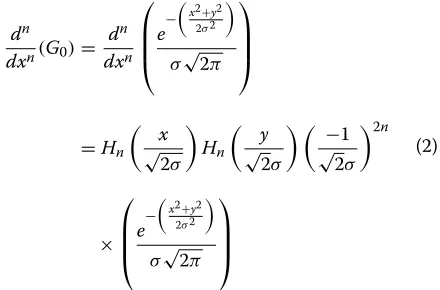
When the differentiation order increases, the Gaussians are fitted and tuned to higher spatial frequencies. Finally, a range of independent channels is constructed.
dn
dxn(G0)=
dn
dxn
⎛ ⎜ ⎜ ⎝e
−
x2+y2 2σ2
σ√2π ⎞ ⎟ ⎟ ⎠
=Hn
x
√
2σ
Hn
y
√
2σ
−1
√
2σ 2n
×
⎛ ⎜ ⎜ ⎝e
−
x2+y2 2σ2
σ√2π ⎞ ⎟ ⎟ ⎠
(2)
The nth Gaussian derivative can be expressed as a Hermite polynomial multiplied by the original Gaussian: (whereσ is the standard deviation of the Gaussian, and the scale factor ensures the function integrates to unity).
2.3 Stage III. steering filtering
The steering stage represents the approach to projecting the space-temporal filters calculated in previous stages under different orientations. Calling nand mthe order inxandydirections, respectively,θ (the angle projected) andD(the derivative operator), the general expression is
derived as a linear combination of filters belonging to the same order basis.
Gθn,m=
n
k=0
n k
(Dxcosθ )k
Dysinθ
n−k
∗
m
i=0
m i
(−Dxsinθ )i
Dycosθ
m−i
G0
(3)
2.4 Stage IV. Taylor truncation
At this stage, a truncated Taylor expansion is per-formed, using each oriented filter previously calculated. This function represents a robust structure that gathers all space-temporal information sequences, approximat-ing one generic pixel by the set of derivatives from the neighborhood, which can be written as follows:
Ix+p,y+q,t+r=
l
i=0
m
j=0
n
k=0 piqjrk
i!j!k!
∗ ∂n
∂xi∂yj∂tkI
x,y,t
(4)
The three Taylor expansion derivatives are constructed in one large image using the completed set of basis fil-ter responses. According to the original model [9], the expansions are truncated after the third-order in the pri-mary direction and the second-order in the orthogonal and temporal directions.
2.5 Stage V. quotients
This is the last stage derived to the common pathway calculation. The next stages implement the modulus and phase estimation with separate expressions. The goal here is to compute a quotient of every sextet’s component:
X=∂I/∂x
Y=∂I/∂y
T=∂I/∂t
→ XX XY XTYY YT TT
→ YTYT//TT XYYY XY//XX XTYY XT//XXTT
(5)
2.6 Stage VI. velocity primitives
The previous stages compute the visual information con-sidering a Taylor representation of each pixel and cal-culating the speed for a range of orientations in order to simulate the orientation columns found in the striate cortex [9]. This is accomplished by rotating the coor-dinate system and Gaussian derivative filters (Steering Stage) to a number of primary directions. Next, the speed measurements–parallel and orthogonal–are placed in pri-mary directions in order to yield a vector of speed mea-surements, whose components are speed and orthogonal speed:
ˆ
s=ˆs,ˆs⊥ (6)
The raw measurements of speed are also conditioned by including the measurements of the image structure
XY/XX and XY/YY, where the final conditioned speed
vectors are given by:
ˆ
s=
2 ⎡ ⎣XT XX 1+ XY XX
2−1⎤ ⎦
ˆ
s⊥=
2 ⎡ ⎣YT YY 1+ XY YY
2−1⎤ ⎦
(7)
is the number of orientations at which speed is evaluated. Inverse speed is also calculated:
˘
s=
2 XT TT ˘
s⊥=
2 YT TT (8)
Inverse speed is evaluated using different terms from those used to compute speed, and so constitutes an additional independent measurement. Finally, the motion modulus is calculated through a quotient of determinants:
Modulus2= ⎡ ⎢ ⎢ ⎢ ⎣ ˆ
scosθ ˆssinθ
ˆ
s⊥cosθ ˆs⊥sinθ
ˆ
s˘s sˆ˘s⊥
ˆ
s⊥˘s sˆ⊥˘s⊥
⎤ ⎥ ⎥ ⎥
⎦ (9)
The direction of motion is extracted by calculating a measurement of phase that is combined across all speed related measurements, since they are in phase:
phase=arctan
˘
s+ ˆssinθ+s˘⊥+ ˆs⊥cosθ
˘
s+ ˆscosθ−˘s⊥+ ˆs⊥sinθ
(10)
3 Multi-criteria motivation for tunning McGM Potential benefits of GPUs in the McGM context have been explored in the literature [14], where authors stud-ied the viability in these novel devices. Throughput results with respect to a single CPU were satisfactory enough in terms of performance, achieving×32 speedups for 2562 resolution movies.
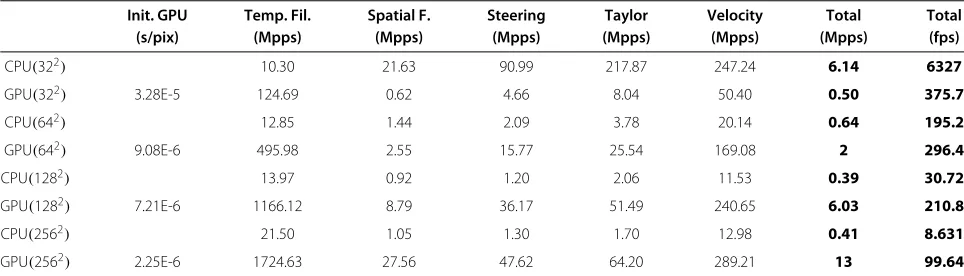
The scope of this study is to explore mechanisms in order to reduce the data amount without losing the efficiency and accuracy requirements. To highlight the memory handicap of GPUs, Table 1 shows the sum-marized performance results observed using the McGM algorithm in a graphic device compared with a single CPU. The performance observed at each stage of the algorithm is shown in Mpixel/s (Mpps), and the global throughput with a particular model configuration, as follows: three temporal derivatives, a temporal convo-lution window of 15 frames, five spatial derivatives, a spatial separable convolution window of 31 pixels, and 12 angles steered. Moreover, as shown in this table, GPU implementation amply fulfilled real-time require-ments in all of the resolution configurations considered. This is further shown in the last column, which cor-responds to overall performance, which was measured in frames per second (fps). While general-purpose pro-cessors can only reach real-time rates for small video resolutions, GPU-based systems enabled higher resolu-tion movies where more DDR memory capacity was available.
In order to reduce algorithm memory consumption, we could afford not to store, as a particular solution, some of the temporary data computations, recalculat-ing when necessary at the expense of reducrecalculat-ing perfor-mance throughput under real time conditions. The most memory-demanding stages in the McGM algorithm cor-respond to the Spatial Filtering and Steering stages. On the one hand, an efficient way to reduce memory neces-sities was to perform the Steering stage with lessθ angles at the expense of accuracy degradation. On the other hand, it was possible to use a numerical derivative [17] instead of the Gaussian counterpart in the Spatial Filtering stage in order to allow faster derivative recalculation. This alternative scheme was based on the fact of not requir-ing intermediate data computation storage by savrequir-ing a huge amount of memory and to recalculate whenever data were used. A simple numerical differentiating filter was
used based on the convolution commutative properties: I⊗Gx = I⊗(G0⊗Dx) = (I⊗G0)⊗Dx. The number
of operations performed in(I⊗G0)⊗Dxare smaller than
the Gaussian derivative filtering, making the convolution process faster.
Table 2 shows the error in computingG0⊗Dx to
eval-uate accuracy degradation. Filter degradation denotes
|(G0⊗DG)−(G0⊗DN)|difference whereDGandDN
cor-responds to Gaussian and Numerical derivative filtering, respectively. As can be appreciated, loss of accuracy is not so important for 9–31 pixel filtering, reaching a maximum of 3% error. A priori, we may conclude that performing numerical derivatives rarely creates considerable error.
Despite the unimportance of degraded filtering accu-racy, an experiment comparing motion estimation degra-dation is carried out to evaluate the loss of accuracy in the overall algorithm. As benchmarks, we have used a cou-ple of synthetic sequences widely accepted in this context: the ‘diverging tree’ and the ‘translating tree’, both created by David Fleet at Toronto University [18]. The ‘diverg-ing tree’ shows an expansive motion of a tree (in camera zoom mode) with an asymmetric velocity range depend-ing on the pixel position (null in the central focus and 1.4 pixels/frame and 2 pixel/frames in the left and right boundaries, respectively). The ‘translating tree’ shows the translational motion of a tree with an asymmetric veloc-ity range depending on the pixel position (zero to 1.73 pixel/frames and zero to 2.3 pixel/frames in the left and right border, respectively). For an error metric, we used Barron [19], considered to be one of the most accepted metrics in the specialized literature.
Barron Equation (11) shows deviation from the correct space-time orientation, the velocity being a 3D unit direc-tion vector. This vector wraps both modulus (speed) and phase (direction) in a single value reducing and reduce the rise of directional errors for small velocities.
v= √ 1
u2+v2+1(u,v, 1)
T (11)
Table 1 Performance of the GPU versus CPU
Init. GPU Temp. Fil. Spatial F. Steering Taylor Velocity Total Total (s/pix) (Mpps) (Mpps) (Mpps) (Mpps) (Mpps) (Mpps) (fps)
CPU(322) 10.30 21.63 90.99 217.87 247.24 6.14 6327
GPU(322) 3.28E-5 124.69 0.62 4.66 8.04 50.40 0.50 375.7
CPU(642) 12.85 1.44 2.09 3.78 20.14 0.64 195.2
GPU(642) 9.08E-6 495.98 2.55 15.77 25.54 169.08 2 296.4
CPU(1282) 13.97 0.92 1.20 2.06 11.53 0.39 30.72
GPU(1282) 7.21E-6 1166.12 8.79 36.17 51.49 240.65 6.03 210.8
CPU(2562) 21.50 1.05 1.30 1.70 12.98 0.41 8.631
Table 2 Filter accuracy degradation using a numerical derivative instead of the Gaussian counterpart for first, second,. . .
to the fifth derivative order
x x x xIV xV
filter degradation 0.003825 0.009415 0.018444 0.033701 0.060134
Since the vector is self-normalized, the angle between the measured velocityveand the correct one vcis given
by Equation (12). This error measurement is calculated for every pixel for which a velocity measurement was recovered.
ψE=arccos(vc·ve) (12)
Table 3 shows an error in Barron’s angle when used as a numerical derivative instead of a Gaussian counter-part in spatial filtering with a significantθ angles reduc-tion in the steering stage. ColumnsO(h), O(h2),O(h3), and O(h4) denote the observed error of Barron’s angle when performed with numerical derivatives with first-, second-, third- and fourth-accuracy order, respectively. #θ is related to the maximum number ofθ angles projected in the Steering stage. The table shows the impact of half-or quarter-θs.
As observed, the ‘diverging tree’ experiment behaves reasonably well with numerical derivatives reducing their impact with a higher order of accuracy. Nevertheless, in the ‘translating tree’ experiment, the algorithm is more vulnerable to numerical derivatives than the number of angles variation. Due to this disparity observed in Table 3, it is advisable the space of feasible solutions with any set of input data be explored. Given the large number of param-eters to configure, on one hand relative to the McGM algorithm, and on the other hand those based on avail-able resources, the use of genetic algorithms (GAs) can be useful to reduce time-consuming exploration.
3.1 Multi-criteria optimization description
The use of GAs arises from non-viability exploration with a large solution space. In our context, the target is to find a compromise in the reduction of the GPU’s mem-ory usage with negligible accuracy degradation that allows motion estimation system self-adaptation under apprecia-ble environmental conditions and changes in a reasonaapprecia-ble time.
The goal of the multi-objective optimization [20] is to simultaneously optimize several objectives that could
be inconsistent. Considering the problems, some trade-offs among the different variables involved also need to be considered. In our context, we consider the following three-objective minimization problem:
Minimize z=f1(x),f2(x),f3(x)
subject to x∈X, (13)
where z is the objective vector with 3 objectives to be minimized: execution timef1, memory usagef2, and loss of accuracyf3;zis the decision vector, andX is the fea-sible region in the decision space, which corresponds to all possible McGM configurations with respect to the derivative decision and the number of angles involved. In GA terminology,xcorresponds to achromosome. In our context:
• Dxcorresponds to the derivative to be computed in
spatial filtering. This information is stored in a two-dimensional array whose values determine the way their derivative is computed by means of Gaussian or order-numerical differentiation. The two-dimensional array position is related to the derivative order.
• The number ofθangles to be performed in the
steering stage, which can be assigned as an integer.
3.2 Our multi-GPU implementation
Over the last few years, a great number of multi-objective evolutionary algorithms have been developed [21-23]. A revision of the GA can be found in a tutorial [24], where the authors provide the revision’s more relevant features.
For this study, we have chosen the NSGA-II [25] for its following advantages:
• Weights are not required, so it is not necessary to study the impact offi(x)and assign them.
• Its computational requirement isone, which presents
less computational complexity.
• Its ‘good’ behavior and ability to find a set of solutions
Table 3 Overall degradation measured as mean absolute error of Barron’s angle
O(h) O(h2) O(h3) O(h4) #θ/2 #θ/4
Diverging tree 0.9297 0.4982 0.4432 0.4020 0.0008 0.0122
near the true Pareto-optimal with few iterations. • It’s widely used and amply tested.
The NSGA-II is based on a fast non-dominated sort-ing procedure where a fast crowded distance estimation is carried out. It involves a simple crowded comparison operator [25]. The NSGA-II algorithm could be summa-rized in the next stages:
1. Initially, a random population is created inpop. 2. The population is sorted based on the
non-domination scheme.
3. It is assigned a fitness, which means every individual of the population is ranked into levels. First-level or Pareto-front is most preferable.
4. A binary tournament selection and combination is carried out.
5. A mutation phase is done.
6. A combined populationR comes from the union of
an oldpopwith the new onenew pop. The
populationR is size2∗pop size.
7. R is ranked by means of the McGM algorithm and
sorted according to a non-domination scheme.
8. New populationpop is made from sizepop size.
The fast non-dominated sorting is the most computa-tional cost part of the GA, because it involves ranking
every individual of the population. We urge that this task be performed entirely on multi-GPUs since this is more efficient than using a CPU, from computational point of view. Most GA operators are executed in CPU due to its low computational demand.
To rank an individual of the population means to compute the McGM algorithm with chromosome configuration, to compute the derivatives in Spatial Filter-ing, and to compute the number of angles in the Steering Stage to be performed. Several levels of parallelism are exploited: a coarser level, where non-dominate sorting is evaluated in parallel on several GPUs, and finer level by means of data parallelism exploitation available in each stage of the McGM algorithm. Algorithm 1 summarizes our parallel implementation where pop size, ngens and
%mutation are GA input parameters which correspond
to population size, number of generations, and muta-tion probability, respectively. The OpenMP paradigm is used to distribute a non-dominated sort across multiple devices by means of#pragma omp parallel fordirectives. Our implementation generates Pareto-optimal solutions with a set of motion estimation execution time, accu-racy pixel error, and GPU memory usage points. This feature allows the choice of one of the best solutions, tak-ing into account the available computational resources favoring the dynamic tuning depending on current conditions.
Algorithm 1 pareto front=multiGPU NSGAII(pop size,ngens, %mutation) pop=random init Population(pop size) %NSGAII−1ststage
Fronts=McGM fast nondominated sort(pop) %NSGAII−2nd&3rdstages
whilegen≤ngensdo
#pragma parallel for shared(Fronts,R) private(i,GPUth,p1,p2) fori=0;i≤pop size;i=i+1do
p1,p2=select parents(pop(i))
newpop(i).x=crossover(p1,p2) %NSGAII−4thstage newpop(i).x=mutation(%mutation) %NSGAII−5thstage R(i)=newpop(i)∪pop(i) %NSGAII−6thstage
GPUth=threadID();
Fronts=McGM fast nondominated sort(GPUth,R(i)) %NSGAII−7thstage
end for k=0
pop= ∅
%NSGAII−8thstage
while sizeof(pop) <pop size do frontk =get fronts(Fronts,k)
pop=pop∪get Relements in front(R,frontk)
k=k+1 end while gen=gen+1 end while
−0.2 −0.1 0 0.1 0.2 0.3 0.4 0.5 0.6 0.7 0.8 20
30 40 50 60 70 80 90 100
Barron´s angle error ΔψE Barron´s angle error ΔψE
% of memory usage
Translating Tree
optimal iter=200 iter=50 iter=20 iter=1
0 0.05 0.1 0.15 0.2 0.25 0.3 0.35 0.4 0.45 0.5 20
30 40 50 60 70 80 90 100
% of memory usage
Diverging Tree
optimal iter=200 iter=50 iter=20 iter=1
Figure 2Evolution of the average objective in the GA for diverging and translating tree sequences.The number of points in the optimal front is a subset of the final solution because execution time components have been removed. This figure shows only 15% of Pareto-pairs for the ‘translating tree’ while those in the ‘diverging tree’ are displayed at 40%.
4 Results
4.1 Work environment
The systems used are based on Tesla technology. The first one consists of 2 Intel Xeon E5645 processors with six cores (2.40 GHz with 12 MB cache memory and Hyper-threading technology) and 2 Tesla M2070 GPUs. The second one is equipped with 2 Quad Intel Xeon E5530 processors (2.40 GHz with 8 MB cache mem-ory and Hyper-threading technology), connecting with 4 Tesla C1060 GPUs. In both cases, the operating sys-tems are Debian 2.6.38 kernels; the compiler used is a GNU g++ v.4.4 with compilation flags-O3 -m64 -fopenmp and CUDA C/C++ SDK v.4.2 with -O3 -fopenmp -arch sm 20/13flags enabled.
The system based on Tesla M2070 incorporates Fermi technology, but due to a scarce number of devices avail-able, a scalability study has been completed with a system based on 4 Tesla C1060 GPUs that allow projections be made of parallel efficiency rates in more modern systems.
4.2 Multicriteria results
Multi-objective GAs are used to look for optimal solutions in a huge search space. In our context, they are employed to achieve a set of optimal solutions that reduce the GPU’s memory usage in the McGM algorithm without losing significant accuracy in the motion estimation scenario. As previously mentioned, the tests were performed using the ‘diverging tree’ and the ‘translating tree’ benchmarks, which are widely accepted in this area.
The first experiment was to evaluate both the conver-gence of the GA and the set of optimal solutions reached. For this purpose, a Euclidean distance metric between consecutive solutions was employed as described in [25]. The GA implemented incorporated a stop condition based on a Euclidean metric when a certain number of
iterations remained invariant to ensure the non-dominant solutions converged to the optimal Pareto-front.
Figure 2 shows the evolution of the set of non-dominated solutions throughout the iterations with a severe stop condition. To facilitate its visualization, only the GPU’s memory reduction and the error difference were included, although the GA also optimizes the motion estimation time. Barron’s angle errorψE corresponds to
the difference of mean Barron error with respect to the original McGM counterpart.
In this experiment, the population size was fixed to 500 with 1% mutation probability. The results obtained indi-cated that after a certain number of generations, the GA barely improved the non-dominant solutions, although it reported new pairs.
Population size only affects the final execution time, achieving results of an optimal solution with similar qual-ity. Empirically, 1% of mutations reported better GA per-formance. Higher mutation rates only suppose significant variations between consecutive generations, which means higher generations are necessary to reach the convergence criterion. Particularly, greater mutation rates suppose a higher number of iterations, which varies between 15 to 320%.
As shown in Figure 2, optimal solutions are gener-ated with significant reduction in memory requirements, achieving even more accurate solutions than the original McGM’s algorithm for the ‘translating tree’ benchmark.
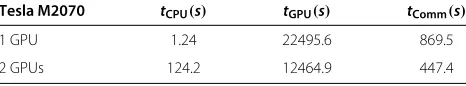
Table 4 Multi-GPU execution times for Tesla M2070 based system
Tesla M2070 tCPU(s) tGPU(s) tComm(s)
1 GPU 1.24 22495.6 869.5
4.3 Multi-GPU results
Table 4 shows GA time measured in seconds in a system based on the Tesla M2070 for the best GA configuration: 1% of mutation rate configuration, 500 individuals and a severe convergence condition to find the Pareto-front. The ‘diverging tree’ was used as a benchmark, although similar performance rates were observed with the ‘trans-lating tree’. Note that the benchmark choice only affects the number of generations processed to reach an opti-mal solution. As expected, the fitness evaluation is the most costly stage of the GA by far. The information exchange overhead between host and devices is not so relevant, which reports satisfactory speedups of×1.79 for 2 GPUs.
Analogous results were obtained in a system with a larger number of graphic devices. Table 5 shows even higher accelerations when 2 GPUs are enabled. Fur-thermore, it is noticeable that scalability rates remain satisfactory with 4 GPUs, achieving ×3.71 speedups. Computational results show that our multi-GPU imple-mentation is efficient in terms of scalability (95 and 93% using 2 and 4 GPUs, respectively), and the tendency indi-cates that GA convergence times would be even lower if more computational resources were available. We can conclude that this successful scalability makes GAs useful for solving problems of this nature. These good perfor-mance results are due to both a well-balanced workload and low overhead involved in data exchange.
Moreover, the use of multiple levels of parallelism reports multiplicative accelerations: first, the speedups achieved in the multi-GPU system, which can be up to
×3.71 with 4 GPUs enabled; and second, the accelera-tions up to ×32 the can be achieved by exploiting the data parallelism on a GPU. On one hand, the combination of both accelerations allows the reduction of exploration time to reach an optimal solution in 99.2% compared with a general-purpose processor. On the other hand, the use of a multi-GPU system not only reports greater FLOPS rates than a CPU, but it is also beneficial in terms of power consumption (MFLOPS/watt).
Moreover, although GA search times are important, their use encourages getting suboptimal solutions that meet the requirements of response time or resource con-sumption, and as GAs evolve, they are gradually refined. This feature, coupled with the chance of a population
Table 5 Multi-GPU execution times for Tesla C1060 based system
Tesla C1060 tCPU(s) tGPU(s) tComm(s)
1 GPU 1.18 23748.0 2025.8
2 GPUs 278.52 12613.1 1022.5
4 GPUs 153.28 6284.4 513.5
size reduction, supposes an impressive simulation times decrease which opens the possibility to build an intelligent system that auto-corrects/adapts depending on the spe-cific requirements or substantial environment changes.
4.4 Visual result
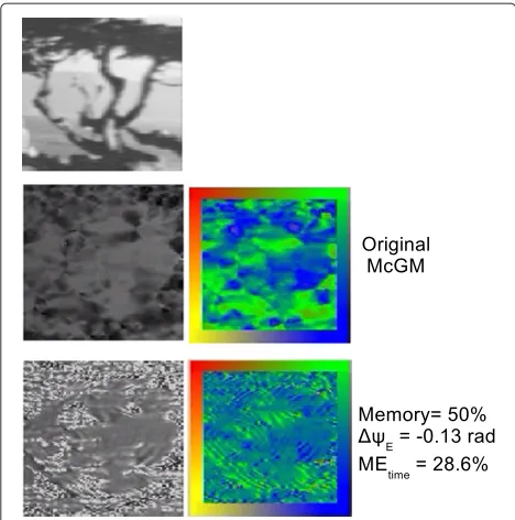
Finally, visual results are presented for both benchmarks considered. Figure 3 shows the main differences in motion estimation outputs in the ‘diverging tree’ benchmark. The original McGM outputs appear at the top of the figure; in the center and at the bottom their counterparts with GA solutions for 75 and 50% memory requirements. It is also remarked the motion estimation time consumption (MEtime). The motion phase (the direction of the pixels) is color-coded from the boundary frame (each particular color pixel points outward to the border color frame). The modulus or velocity magnitude is represented by a lin-ear intensity of gray scales. Similarly, Figure 4 displays GA solutions for the ‘translating tree’ benchmark.
For the ‘diverging tree’, a reduction of 75% in mem-ory usage returns the same precision using the Barron metric and 50% of the McGM execution time (MEtime)
Figure 3The temporal blur of the original stimulus, modulus, and motion phase with the original McGM algorithm (top), and a
Figure 4The temporal blur of the original stimulus, modulus, and motion phase with the original McGM algorithm (top), and a
zGA solution of 50% (bottom) of memory usage for the ‘translating tree’.
compared to the original algorithm. However, the config-uration that reduces memory usage by 50% degrades the accuracy in 22% with a speedup of×3.3.
For ‘translating tree’ benchmark, a solution with half of memory requirements is more accurate (Barron’s error is 0.13 radians less than the original McGM) and×3.5 faster. Despite Barron metric’s popularity by the scientific community in the context of motion estimation, some authors [26,27] point out specific performances due to its asymmetry and its bias of large flow vectors.
4.5 Other error metrics
Although Barron’s metric [19] is probably the most used in the motion estimation scope, there are other metrics used by Machine Vision community that must be taken into account in order to enhance the visibility and generality of the results obtained.
Otte and Nagel [26,27] remarked the fact of asymme-try and bias for extensive optical-flow vectors. Based on this drawback, it is proposed a new metric which accounts the magnitude difference between bidimensional ground truth flow vector (ofvc) and the estimated one (ofve) as
shown in the Equation (14):
O&N =ofvˆc− ˆofve (14)
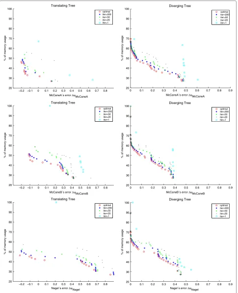
McCane et al. [27] claims this is not sufficient due it gets discount error in regions of small flows. They propose two metrics in order to overcome these problems. The first
metric is the angle difference between the correct tridi-mensionalvcvector and the estimated oneveused in the
Barron’s metric (Equation (15)) but the third component is replaced byδ. In our experiments we assignδ=0.75. This threshold modulates the error considering less significant in zones of small flow than in zones of large flow.
McCaneA =cos−1(vˆc,vˆe) (15)
An additional metric is proposed, such as the normalize magnitude of the vector difference between the estimated and the correct tridimensional flow vectors. The normal-ization factor is the magnitude of the correct flow, it is taken into account the effect of small flows using a signifi-cance thresholdTas shown in Equation (16). It is choseT to be 0.5 pixels. The effect of this threshold would result in a normalized error equal to the unity.
McCaneB =
⎧ ⎪ ⎨ ⎪ ⎩
vc−ve
vc if vc ≥T
ve−T
T if vc<T≤ ve
0 if vc<T>ve
(16)
Figure 5 shows the trend of the NSGA-II algorithm con-sidering McCane and Otte&Nagel metrics. Analogously to Section 4.2, ‘translating’ and ‘diverging tree’ sequences are also used as benchmarks.
For the sake of clarity, Table 6 summarizes the main suc-cessful configuration reported by GA execution. Results observed are consistent with regardless of the metric used. Meanwhile for ‘translating tree’ improves Motion Estimation effectiveness with a significant reduction of memory requirements, for ‘diverging tree’ no degrada-tion is observed for 75% memory usage for any metric performed. From the viewpoint of the execution times, performance results are as expected. On the one hand a reduction in memory requirements by 50% are trans-lated into speedups from 3.3×to 4×. On the other hand, 75% of memory consumption reports an average of 50% in motion estimation execution time.
5 Conclusions
A new and highly parallel approach is presented to over-come the GPU memory usage problems that occurred in our previous implementation of a well-known neuromor-phic motion estimation algorithm. This context provides the main motivation for using evolutionary algorithms to solve multi-criteria optimization problems. The use of GAs based on a multi-GPU scheme allowed for quick exploration of feasible solutions with any set of input data. The choice of NSGA-II is motivated by the good results observed in a few iterations and a near-optimal Pareto-front.
−0.2 −0.1 0 0.1 0.2 0.3 0.4 0.5 0.6 0.7 0.8 20
30 40 50 60 70 80 90 100
McCaneA´s error ΔψMcCaneA
−0.2 −0.1 0 0.1 0.2 0.3 0.4 0.5 0.6 0.7 0.8 McCaneB´s error ΔψMcCaneB
−0.2 −0.1 0 0.1 0.2 0.3 0.4 0.5 0.6 0.7 0.8
McCaneA´s error ΔψMcCaneA
% of memory usage
20 30 40 50 60 70 80 90 100
% of memory usage
20 30 40 50 60 70 80 90 100
% of memory usage
20 30 40 50 60 70 80 90 100
% of memory usage
Translating Tree
optimal iter=200 iter=50 iter=20 iter=1
0 0.1 0.2 0.3 0.4 0.5 0.6 0.7 0.8 0.9
McCaneB´s error ΔψMcCaneB 20
30 40 50 60 70 80 90 100
% of memory usage
0 0.1 0.2 0.3 0.4 0.5 0.6 0.7 0.8 0.9
20 30 40 50 60 70 80 90 100
% of memory usage
0 0.1 0.2 0.3 0.4 0.5 0.6 0.7 0.8 0.9 Diverging Tree
optimal iter=200 iter=50 iter=20 iter=1
Translating Tree
optimal iter=200 iter=50 iter=20 iter=1
Diverging Tree
optimal iter=200 iter=50 iter=20 iter=1
Translating Tree
optimal iter=200 iter=50 iter=20 iter=1
Nagel´s error ΔψNagel Nagel´s error ΔψNagel
Diverging Tree
optimal iter=200 iter=50 iter=20 iter=1
Figure 5Evolution of the average objective in the GA for Diverging and Translating Tree sequences for McCane and Otte&Nagel metric.
Table 6 Best configuration achieved for a reduction of 75 and 50% memory requirements using McCane and Otte&Nagel metric
Error metric Benchmark Memory MEtime Accuracy
(ψ)
Barron ‘Translating tree’ 50% 28.6% −0.13
‘Diverging tree’ 75% 50.0% 0.00
50% 33.3% 0.05
McCaneA ‘Translating tree’ 50% 26.9% −0.12
‘Diverging tree’ 75% 49.1% 0.00
50% 28.9% 0.05
McCaneB ‘Translating tree’ 50% 29.6% −0.11
‘Diverging tree’ 75% 49.2% 0.00
50% 34.5% 0.09
Otte&Nagel ‘Translating tree’ 50% 25.3% −0.21
‘Diverging tree’ 75% 49.1% 0.00
50% 35.7% 0.12
• For ‘diverging tree’, a reduction of 75% in memory usage returns the same precision as the all metrics considered and 50% of the McGM execution time compared to the original algorithm. A configuration that reduces memory usage by 50% degrades the accuracy from 15 to 25% with a range of speedup which varies from×2.8to×3.5.
• For ‘translating tree’, a configuration that has half of the memory requirements is more accurate in terms of error and is between×3.3to×4faster.
From the point of view of multi-GPU efficiency is observed:
• Successful performance of×3.71speedups are
archived when four GPUs are enabled.
• Our implementation is a scalable approach due to
both a well-balanced workload and low-impact communication between host and device.
• A found multiplicative effect:×3.71speedups in a
multi-GPU system by×32acceleration by means of
exploiting the data parallelism on a GPU. An impressive GA time in reaching an optimal solution in 99.2% compared with a CPU.
• An alternative to be considered in terms of power
consumption (MFLOPS/watt).
Because of these encouraging results, the possibil-ity exists for building an intelligent system that auto-corrects/adapts depending on specific requirements or environmental condition variations as the GA evolves.
Future lines are based on reusing this system with an environment predictor, with the possibility of real-time execution and self reconfiguration depending on
the external constraints and resources available in the platform. This system is expected to contribute to the new machine vision trends, useful for many real-world applications.
Competing interests
The authors declare that they have no competing interests.
Acknowledgements
The present study had been supported by Spanish Projects CICYT-TIN 2008/508, CICYT-TIN 2012-32180 and Ingenio Consolider ESP00C-07-20811.
Received: 31 October 2012 Accepted: 14 December 2012 Published: 19 February 2013
References
1. M Shaaban, S Goel, M Bayoumi, Motion estimation algorithm for real-time systems. IEEE Workshop on Signal Processing Systems, 257–262 (2004) 2. JY Kang, S Gupta, S Shah, JL Gaudiot, An efficient pim
(processor-in-memory) architecture for motion estimation, IEEE International Conference on Application-Specific Systems. Architectures, and Processors, 282–292 (2003)
3. JY Kang, S Gupta, JL Gaudiot, An efficient data-distribution mechanism in a processor-in-memory (pim) architecture applied to motion estimation. IEEE Trans. Comput.57(3), 375–388 (2008)
4. HS Oh, HK Lee, Block-matching algorithm based on an adaptive reduction of the search area for motion estimation. Real-Time Imag.6(5), 407–414 (2000)
5. CL Huang, YT Chen, Motion estimation method using a 3d steerable filter. Image Vis. Comput.13(1), 21–32 (1995)
6. S Baker, R Gross, I Matthews, Lucas-kanade 20 years on: a unifying framework: Part 3. Int. J. Comput. Vis.56, 221–255 (2002)
7. YM Chi, TD Tran, R Etienne-Cummings, Optical flow approximation of sub-pixel accurate block matching for video coding. IEEE ICASSP.1, 1017–1020 (2003)
8. A Johnston, PW McOwan, CP Benton, A unified account of three apparent motion illusions. Vis. Res.35(8), 1109–1123 (1995)
9. PW McOwan, CPB, A Johnston, Robust velocity computation from a biologically motivated model of motion perception. Proc. Royal Soc. B. 266, 509–518 (1999)
10. X Liang, PW McOwan, A Johnston, Biologically inspired framework for spatial and spectral velocity estimations. J. Opt. Soc. Am. A.28(4), 713–723 (2011)
11. G Botella, A Garc´ıa, M Rodriguez-Alvarez, E Ros, U Meyer-Bˆase, MC Molina, Robust bioinspired architecture for optical-flow computation. IEEE Trans. VLSI Syst.18(4), 616–629 (2010)
12. L Mattes, S Kofuji, Overcoming the GPU memory limitation on FDTD through the use of overlapping subgrids. Int. Conference on Microwave and Millimeter Wave Technology, 1536–1539 (2010)
13. Y Zhou, M Garland, Interactive point-based rendering of higher-order tetrahedral data. IEEE Transactions on Visualization and Computer Graphics.12(5), 1229–1236 (2006)
14. F Ayuso, G Botella, C Garcia, M Prieto, F Tirado, GPU-based acceleration of bioinspired motion estimation model. Concurrency and Computation: Practice and Experience p. (in press). doi:10.1002/cpe.2946 (2012) 15. RJ Snowden, RF Hess, Temporal frequency filters in the human peripheral
visual field. Vis. Res.32(1), 61–72 (1992)
16. JJ Koenderink, Optic flow. Vision Research.26, 161–180 (1996) 17. B Fornberg, Generation of finite difference formulas on arbitrarily spaced
grids. Math. Comput.51(184), 699–706 (1988)
18. DJ Fleet,Measurement of Image Velocity. (Kluwer Academic Publishers, Norwell, MA, USA, 1992)
19. JL Barron, DJ Fleet, SS Beauchemin, Performance of optical flow techniques. Int. J. Comput. Vis.12, 43–77 (1994)
20. A Konak, D Coit, D Smith, Multi-objective optimization using genetic algorithms: a tutorial. Reliab. Eng. Syst. Safety.91(9), 992–1007 (2006) 21. C Fonseca, P Fleming, Genetic algorithms for multiobjective optimization:
22. N Srinivas, K Deb, Muiltiobjective optimization using nondominated sorting in genetic algorithms. Evol. Comput.2(3), 221–248 (1994) 23. CA Coello Coello, inComputational Intelligence: Principles and Practice,
chap. 4, ed. by GY Yen, DB Fogel. 20 years of evolutionary multi-objective optimization: what has been done and what remains to be done (IEEE Computational Intelligence Society, Vancouver, Canada, 2006), pp. 73–88. ISBN 0-9787135-0-8
24. E Zitzler, M Laumanns, S Bleuler, A tutorial on evolutionary multiobjective optimization. In Metaheuristics for Multiobjective Optimisation (Springer-Verlag).535, 3–38 (2003)
25. K Deb, A Pratap, S Agarwal, T Meyarivan, A fast elitist multi-objective genetic algorithm: Nsga-ii. IEEE Trans. Evol. Comput.6, 182–197 (2000) 26. M Otte, HH Nagel, Estimation of optical flow based on higher-order
spatiotemporal derivatives in interlaced and non-interlaced image sequences. Artif. Intell.78(1), 5–43 (1995)
27. B McCane, K Novins, D Crannitch, B Galvin, On benchmarking optical flow. Comput. Vis. Image Underst.84(1), 126–143 (2001)
doi:10.1186/1687-6180-2013-23
Cite this article as:Garciaet al.:Multi-GPU based on multicriteria optimiza-tion for mooptimiza-tion estimaoptimiza-tion system.EURASIP Journal on Advances in Signal Processing20132013:23.
Submit your manuscript to a
journal and benefi t from:
7Convenient online submission
7Rigorous peer review
7Immediate publication on acceptance
7Open access: articles freely available online
7High visibility within the fi eld
7Retaining the copyright to your article