New Possibilities and Applications of the Least Squares
Collocation Method
VasiliyShapeev1,2,,VasiliyBelyaev1,,SergeyGolushko2,3,, and
SemyonIdimeshev3,
1Institute of Theoretical and Applied Mechanics of SB RAS 2Novosibirsk State University
3Institute of Computational Technologies of SB RAS
Abstract.Least squares collocation method (LSC) is a versatile numerical method for solving boundary value problems for PDE. The present article demonstrates the abilities of LSC to solve various problems – in particular, calculations of bending of isotropic irregular shaped plates and multi-layered anisotropic plates. In order to achieve higher accuracy, new versions of the method utilize high-degree polynomial spaces. The numer-ical experiments demonstrate high accuracy of the solutions.
1 Introduction
The least squares collocation method (LSC), as the name suggests, is a combination of two methods. In LSC, the initial differential problem
Lu(x)=f(x), x∈Ω (1)
with boundary conditions
lu(x)=g(x), x∈∂Ω (2)
is projected by collocation into a finite-dimensional functional space. Different polynomial spaces are often used as functional spaces. Here, Landldenote differential operators,u =(u1,u2, . . . ,um)
— unknown vector function,x=(x1,x2, . . . ,xn),x1,x2, . . . ,xn— independent variables, f andg—
given vector functions.
The approximate solutionua(x) of the problem (1), (2) is represented as a linear combination of
basis elementsφi(x) of selected functional space with unknown coefficientsci:
ua(x)= N
i=1
ciφi(x). (3)
If the initial problem is nonlinear, we can utilize linearization and include nonlinearity iterations in algorithm. Therefore, (1) and (2) are considered as linear onwards.
The domainΩis covered by a grid, with a local solution required for each grid cell. Similarly to collocation method, in order to define a local solution, collocation equations are obtained by substi-tuting (3) into (1) at given pointsxc ∈Ω. Boundary conditions are obtained by substituting (3) into
(1) at given pointsxb ∈∂Ω. Additionally, LSC requires matching conditions (MC) between solutions
in neighbor cells. Matching conditions must not contradict the definition of problem solution. Choice of MC type is up to the mathematician. An example of MC are continuity requirements for analytical relationslm(u)=0 defined at selected pointsxmon common sides of neighbor cells. Thus, the system
of linear algebraic equations (SLAE) for unknown coefficientsc=(c1, . . . ,cN) is constructed of
col-location equationsLua(xc)=f(xc), boundary conditionslua(xb)=g(xb), and matching conditions. In
order to define a local solution in each cell, an overdetermined (local) SLAEAec=bewith a
rectan-gular full-rankM×NmatrixAe, (M >N) must be formed. The set of all local SLAE produces the
global SLAEAc=b. The matrix of this global SLAE is coarse, therefore, algorithms that take matrix coarseness into consideration are best suited for its solution. In practice, for the global SLAE solution, it is convenient to use an iteration process based on direct methods for the local SLAE. In order to do this, all cells of the domain are sequentially processed in one “global” iteration, and in each cell, local SLAE are solved with direct methods. During this process, coefficientscin neighbor cells can be taken from the previous global iteration (Gauss-Jacobi process) or current iteration (Gauss-Seidel process). Implemented versions of LSC are further detailed in [1, 2, 7–10].
Several methods can be used to solve the corresponding linear least squares problem. Within the normal equations method, we define a vector ˇcfrom the set of all possible pseudosolutions of the overdetermined systemAec=beas a solution of the systemAeTAecˇ=ATebwith normal (symmetrical
and positive-definite) matrixA1 = ATeAe. The solution obtained in this way minimizes the residue
functionalΦ = Mj=1(rj)2 on the set of all possible pseudosolutions of Aec =be. Here, the residue
r = (r1, . . . ,rM) ≡ Aec−be. The same solution ˇcof system Aec = be can also be found by QR
decomposition of the matrix Ae. In order to achieve this, we use conventional methods to find an
orthogonal matrixQsuch that the firstNrows of the matrixRe=QAewould form the upper triangular
matrixR; the solution is then found by solving the firstNequations of the systemRec=Qbe. Ifνis
the matrix condition number, the following relations hold:ν(A1)=ν2(Ae) andν(QAe)=ν(Ae). Thus,
if the SLAE is ill-conditioned, the second method is favorable. This circumstance was systematically taken into account during the development of LSC versions for solving various types of problems.
If the initial problem is nonlinear, we can utilize linearization and include nonlinearity iterations in algorithm. Therefore, (1) and (2) are considered as linear onwards.
The domainΩis covered by a grid, with a local solution required for each grid cell. Similarly to collocation method, in order to define a local solution, collocation equations are obtained by substi-tuting (3) into (1) at given points xc ∈Ω. Boundary conditions are obtained by substituting (3) into
(1) at given pointsxb∈∂Ω. Additionally, LSC requires matching conditions (MC) between solutions
in neighbor cells. Matching conditions must not contradict the definition of problem solution. Choice of MC type is up to the mathematician. An example of MC are continuity requirements for analytical relationslm(u)=0 defined at selected pointsxmon common sides of neighbor cells. Thus, the system
of linear algebraic equations (SLAE) for unknown coefficientsc=(c1, . . . ,cN) is constructed of
col-location equationsLua(xc)= f(xc), boundary conditionslua(xb)=g(xb), and matching conditions. In
order to define a local solution in each cell, an overdetermined (local) SLAEAec=bewith a
rectan-gular full-rankM×NmatrixAe, (M >N) must be formed. The set of all local SLAE produces the
global SLAEAc=b. The matrix of this global SLAE is coarse, therefore, algorithms that take matrix coarseness into consideration are best suited for its solution. In practice, for the global SLAE solution, it is convenient to use an iteration process based on direct methods for the local SLAE. In order to do this, all cells of the domain are sequentially processed in one “global” iteration, and in each cell, local SLAE are solved with direct methods. During this process, coefficientscin neighbor cells can be taken from the previous global iteration (Gauss-Jacobi process) or current iteration (Gauss-Seidel process). Implemented versions of LSC are further detailed in [1, 2, 7–10].
Several methods can be used to solve the corresponding linear least squares problem. Within the normal equations method, we define a vector ˇcfrom the set of all possible pseudosolutions of the overdetermined systemAec=beas a solution of the systemAeTAecˇ=ATebwith normal (symmetrical
and positive-definite) matrix A1 = ATeAe. The solution obtained in this way minimizes the residue
functionalΦ =Mj=1(rj)2 on the set of all possible pseudosolutions of Aec = be. Here, the residue
r = (r1, . . . ,rM) ≡ Aec−be. The same solution ˇcof system Aec = be can also be found by QR
decomposition of the matrix Ae. In order to achieve this, we use conventional methods to find an
orthogonal matrixQsuch that the firstNrows of the matrixRe=QAewould form the upper triangular
matrixR; the solution is then found by solving the firstNequations of the systemRec=Qbe. Ifνis
the matrix condition number, the following relations hold:ν(A1)=ν2(Ae) andν(QAe)=ν(Ae). Thus,
if the SLAE is ill-conditioned, the second method is favorable. This circumstance was systematically taken into account during the development of LSC versions for solving various types of problems.
Presently, different LSC versions are implemented for various PDE system types, with different approximation orders, with regular and irregular grids including irregular domains, using multi-grid complexes, preconditioners, Krylov subspaces, utilizing varied polynomial spaces, different matching conditions. We simultaneously investigated method properties and applicability for problems with sin-gularities, comparing numerical results with those published by other authors and found in benchmark problems. LSC has been successfully used in solving problems of viscous flow in cavities, calculat-ing 3D thermophysical processes in laser weldcalculat-ing of plates made of homogeneous and heterogeneous metals (including multi-layer composite insets), calculating stress in isotropic and anisotropic plates of various shapes, plates and rectangular beams made of composite materials, and so on. We briefly explain some of the aforementioned and new results.
2
p
- and
hp
- versions of LSC method
Each cell of the gridΩi, (i =1, . . . ,K) has local coordinates for convenience, e.g. in case of a 2D
domain:
ξ1= x1−x
∗
1
h , ξ2=
x2−x∗2
h .
For a grid with rectangular cells (x∗
1,x∗2) is cell center;h =(h1h2)1/2– cell dimensions alongx1,x2
axes, respectively. We will use the termh-version of LSC if the grid has a great number of cells and the solution representation for (3) has a small number of basis elements. Conversely, ap-version of LSC has a single cell with possibly many basis elements in the representation (3). Initially, the researchers used and studiedh-versions of LSC for solving mathematical physics equations and Navier-Stokes equations; these versions had small degree of basis polynomials [1], but sufficient for the approx-imation of (1), (2). However, achieving good solution accuracy usingh-version with low approxi-mation order requires substantially finer grids and respectively large SLAE. The inevitable rounding error accumulation significantly limits the potential ofh-versions of LSC. p-versions of the method (pseudospectral versions) were later examined [7]: the domain consisted of one cell, and various high-degree polynomials were used to achieve acceptable solution accuracy. Numerical experiments showed that using p-versions may yield acceptable solution accuracy for applied problems, e.g. lay-ered fluid flow, isotropic and anisotropic plate strength. However, if solution smoothness is limited, usage ofp-version may be inefficient. Variants ofhp-versions of LSC are most practical when used with moderate values of basis polynomial degrees and a moderate number of grid cells. They are more flexible and efficient thanh- andp-versions.
Let us demonstrate the above by solving the Dirichlet problem for the Poisson equation:
∂2u(x1,x2)
∂x2 1
+∂
2u(x 1,x2)
∂x2 2
=∂
2u
ex(x1,x2)
∂x2 1
+∂
2u
ex(x1,x2)
∂x2 2
, (4)
u(x1,x2)=uex(x1x2), (x1,x2)∈∂Ω, Ω =[−1; 1]×[−1; 1].
The exact solution is a product of functions from Runge’s example [3]:
uex(x1,x2)= 1
(1+25x21) 1
(1+25x22). (5)
The approximate solutionua(x1,x2) has a form
ua(ξ1, ξ2)=
N1−1
i=0
N2−1
j=0
ci jTi(ξ1)Tj(ξ2), (ξ1, ξ2)∈[−1; 1]×[−1,1], (6)
whereTi(ξ) –i-th degree Chebyshev polynomials. The roots of polynomials serve as coordinates for
collocation, matching, and boundary points. Usage of p-version (single cell) with N1 = N2 =100 allowed to achieve a solution inC-norm with errorEc =1.96·10−7, whereashp-version with only
four cells andN1=N2=25 led to errorEc=3.10·10−14. The advantage of thehp-version over the
h-version was noticed while attempting to improve solution accuracy of the benchmark problem of viscous flow inside a square cavity with Reynolds number within the interval [1000; 7500]. Numerical experiments conducted on hp-version with a monomial basis (max degree 6) and Re=1000 yielded solution accuracy of≈10−8. This was determined after a large number of numerical experiments and
3 Application of LSC method to calculation of stress and displacement
fields in composite plates
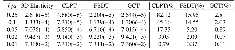
Stress and displacement fields calculation in composite constructions and elements is an important problem for various industries. Numerical modeling in this field of knowledge often allows to sub-stitute physical experiments, thus accelerating and cheapening the development of new materials and constructions. Researching strength properties of multi-layered composite plates under load often requires stress and displacement fields calculation. Assume that the plate layers consist of materials with different strength properties, and these materials are in elastic state. Such calculation can be per-formed by means of 3D elasticity theory. This approach requires solving a complex resource-intensive problem, i.e. solving a system of 3D equations for every layer while considering interaction condi-tions between layers. Solving this kind of problem requires significant computational power, which considerably lowers the effectiveness of numerical modeling. To solve this problem with a desktop computer, instead of 3D elasticity theory, we suggest using its 2D approximations. We use three composite plate theories: classical laminated plate theory (CLPT) [4], first shear deformation theory (FSDT) [4], and Grigolyuk-Chulkov theory (GCT) [5]. It is necessary to define their accuracy if pos-sible and evaluate their applicability area. Therefore, the numerical method must not add any error to PDE solution greater than the error of the observed models. In order to evaluate the applicability of each model, results were compared to those derived from 3D elasticity theory. In particular, for bending problem of three-layered plate under uniform load [6]. A substantial number of calculations has been performed. Results of one of them are demonstrated in table 3.
Table 1.Values of bending functions in the center of a three-layered plate, calculated using 4 models: 3D elasticity theory, classical laminated plate theory (CLPT), first shear deformation theory (FSDT), Grigolyuk-Chulkov theory (GCT). Considered plates have varied thicknessh/a,h– thickness,a– characteristic
size in plate plane. The three right columns show percentage difference of bending values in each plate theory
model relative to 3D elasticity theory model.
h/a 3D Elasticity CLPT FSDT GCT CLPT(%) FSDT(%) GCT(%)
0.25 2.618(−5) 4.680(−6) 2.200(−5) 2.544(−5) 82.12 15.95 2.81 0.1 1.333(−4) 7.310(−5) 1.139(−4) 1.306(−4) 45.16 14.55 2.02 0.05 7.078(−4) 5.850(−4) 6.710(−4) 7.015(−4) 17.35 5.20 0.89 0.02 9.427(−3) 9.140(−3) 9.230(−3) 9.421(−3) 3.05 2.09 0.07 0.01 7.368(−2) 7.310(−2) 7.341(−2) 7.360(−2) 0.79 0.37 0.11
4 Solving boundary value problems for PDE in irregular domains with
high-order accuracy
3 Application of LSC method to calculation of stress and displacement
fields in composite plates
Stress and displacement fields calculation in composite constructions and elements is an important problem for various industries. Numerical modeling in this field of knowledge often allows to sub-stitute physical experiments, thus accelerating and cheapening the development of new materials and constructions. Researching strength properties of multi-layered composite plates under load often requires stress and displacement fields calculation. Assume that the plate layers consist of materials with different strength properties, and these materials are in elastic state. Such calculation can be per-formed by means of 3D elasticity theory. This approach requires solving a complex resource-intensive problem, i.e. solving a system of 3D equations for every layer while considering interaction condi-tions between layers. Solving this kind of problem requires significant computational power, which considerably lowers the effectiveness of numerical modeling. To solve this problem with a desktop computer, instead of 3D elasticity theory, we suggest using its 2D approximations. We use three composite plate theories: classical laminated plate theory (CLPT) [4], first shear deformation theory (FSDT) [4], and Grigolyuk-Chulkov theory (GCT) [5]. It is necessary to define their accuracy if pos-sible and evaluate their applicability area. Therefore, the numerical method must not add any error to PDE solution greater than the error of the observed models. In order to evaluate the applicability of each model, results were compared to those derived from 3D elasticity theory. In particular, for bending problem of three-layered plate under uniform load [6]. A substantial number of calculations has been performed. Results of one of them are demonstrated in table 3.
Table 1.Values of bending functions in the center of a three-layered plate, calculated using 4 models: 3D elasticity theory, classical laminated plate theory (CLPT), first shear deformation theory (FSDT), Grigolyuk-Chulkov theory (GCT). Considered plates have varied thicknessh/a,h– thickness,a– characteristic
size in plate plane. The three right columns show percentage difference of bending values in each plate theory
model relative to 3D elasticity theory model.
h/a 3D Elasticity CLPT FSDT GCT CLPT(%) FSDT(%) GCT(%)
0.25 2.618(−5) 4.680(−6) 2.200(−5) 2.544(−5) 82.12 15.95 2.81 0.1 1.333(−4) 7.310(−5) 1.139(−4) 1.306(−4) 45.16 14.55 2.02 0.05 7.078(−4) 5.850(−4) 6.710(−4) 7.015(−4) 17.35 5.20 0.89 0.02 9.427(−3) 9.140(−3) 9.230(−3) 9.421(−3) 3.05 2.09 0.07 0.01 7.368(−2) 7.310(−2) 7.341(−2) 7.360(−2) 0.79 0.37 0.11
4 Solving boundary value problems for PDE in irregular domains with
high-order accuracy
Lately, mathematical modeling specialists have concluded that development of new methods with high-order accuracy is required, due to the necessity of modeling complex physical processes. In particular, high accuracy numerical methods are required for solving problems in irregular domains, since most simulated physical processes take place in such domains. Development of these methods based on conventional methods is impossible or significantly difficult. For instance, in finite diff er-ence methods, a boundary condition related to boundary points is assigned to nearest grid nodes not located on boundary. An error of orderO(h) is thus brought into the finite difference solution. In many cases, the approximation order of the solution is rarely higher than 1. With relative ease, the LSC method allows an approximation of the problem (1), (2) with high-order accuracy in variously
shaped domains. Its evident property is that the approximate solution inside each grid cell is not strictly dependent on the cell shape. This allows to select a single layer of variously shaped cells near domain boundary and approximate the boundary conditions at pointsxbwhich are located exactly on
the boundary∂Ω. The above feature gives an opportunity to avoid the irremovable error related to shifting points away from boundary. Obviously, working with variously shaped cells complicates the algorithm for the problem (1), (2) approximation. Different implemented versions of these algorithms have relatively varied solution accuracy for the same domain. Since it is not possible to describe them in detail here, we only point out their characteristic features which are also used in other methods. For example, it became apparent that using a regular grid within the domainΩis advisable in versions with rectangular cells implemented in [9, 10]. In this case, the transition from cell to cell during calculations is done by simply shifting the index (cell number) by 1. Therefore, there is no need to store neighbor position for every cell in computer memory or use search algorithms based on graph theory. The latter complicates working program algorithms and increases solution time, as specialists point out. Let the cell intersected by the domain boundary∂Ωbe called boundary cell; its part within Ωis called the irregular cell (IC), and its part outsideΩis the extraboundary part.
Table 2.N1×N2— grid size,Niter— number of iterations
N1×N2 Ec Niter log2
EN1/2,N2/2
EN1,N2
10×10 8.19·10−9 63 —
20×20 3.41·10−10 120 4.58
40×40 1.75·10−11 321 4.28
80×80 3.92·10−13 729 4.48
LSC algorithms that utilize extraboundary parts, i.e. collocation points within them (typeI algo-rithms), are simpler than algorithm versions which use only irregular cells (typeIIalgorithms). The technique of grid refinement in multiple numerical experiments in various domains shows that like in other methods, using elongated cells and small cells next to larger cells decreases solution accuracy. A formal check for cell size was included in automated grid building programs. Small IC in type II
Figure 1. The numerical domain (grid size is 5×5). The symbol•denotes the collocation points;×— the matching points;— the points for recording the boundary condi-tions. The triangle IC 5 joins with the cell 6, the IC 14 and 18 join with the IC 13, the IC 20 joins with the cell 16.
algorithms were automatically joined to nearest regular or irregular cells. A unified solution was then found for such joined cells. Mixed type algorithms which are more flexible than type I and II have also been implemented. A sample grid built with mixed algorithm is displayed in figure 1. Presently, three types of algorithms have been implemented which use 2nd, 4th, 8th degree polynomial spaces for solving the Dirichlet problem for the Poisson equation over arbitrary triangular and convex quadri-lateral domains (figure 1), and a domain with curvilinear boundary comprised of smooth curve pieces [9, 10]. A curvilinear boundary domain is represented either as a set of joined analytic-form curve pieces, or a discrete set of points located on the boundary (figure 2). In the latter case, the program builds a continuous spline (x1(t),x2(t)) if boundary is smooth, or a piece-wise spline if boundary has
breakpoints.
An example of discretely defined domain boundary can be seen in figure 2. We used it to verify convergence of numerical solution of the Dirichlet problem for the Poisson equation. Functions with-out singularities were used as boundary conditions in this example. Numerical experiments performed on a sequence of refining grids demonstrated high convergence order of numerical solution for prob-lems without singularities. The regular cell size was formally used as cell size within the sequence. Tests show that the solution of a well-conditioned differential problem with high-degree polynomials has a high convergence order, and its accuracy on relatively coarse grids is close to the accuracy of the computer number representation. Results for solving the Dirichlet problem for the Poisson equa-tion with test soluequa-tionu(x1,x2) =ex1+ex2over the quadrilateral domain with vertices (0,0), (1,0),
(0.8,0.3), (−0.3,0.9) are shown in table 2. LSC method with 4th degree polynomial space was used
in this case. The table demonstrates a convergence order not less than 4.
For stress and displacement fields calculation of variously shaped isotropic plates, we imple-mented mixed type algorithms using 4th degree polynomial space for solving the biharmonic equation in irregular domains. Plate deflection value is defined by the solution of the biharmonic equation
∂4w(x1,x2)
∂x4 1
+2∂
4w(x 1,x2)
∂x2 1∂x22
+∂
4w(x 1,x2)
∂x4 2
= q(x1,x2)
D , (x1,x2)∈Ω. (7)
In (7), w(x1,x2) denotes the deflection of plate midplane, q(x1,x2) – the transverse load, D =
Eh3/12(1−ν2) – the plate rigidity under bending,h – the plate thickness, E, ν– Young’s module
and Poisson ratio of isotropic plate material, domain Ω – the midplane. The following boundary conditions may be specified for plate edges:
w=0, ∂w
∂n =0 — clamped edge; (8)
w=0, Mnw=0 — simply-supported edge; (9)
Mnw=0, Vnw=0 — free edge. (10)
Here,nis the external normal to domain boundary∂Ω,Mn– the second order differential operator,Vn
– the third order differential operator [12].
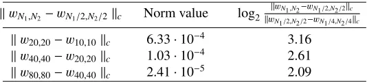
Table 3.Results of numerical experiments
wN1,N2−wN1/2,N2/2c Norm value log2
wN1,N2−wN1/2,N2/2c
wN1/2,N2/2−wN1/4,N2/4c
w20,20−w10,10c 6.33·10−4 3.16
w40,40−w20,20c 1.03·10−4 2.61
algorithms were automatically joined to nearest regular or irregular cells. A unified solution was then found for such joined cells. Mixed type algorithms which are more flexible than type I and II have also been implemented. A sample grid built with mixed algorithm is displayed in figure 1. Presently, three types of algorithms have been implemented which use 2nd, 4th, 8th degree polynomial spaces for solving the Dirichlet problem for the Poisson equation over arbitrary triangular and convex quadri-lateral domains (figure 1), and a domain with curvilinear boundary comprised of smooth curve pieces [9, 10]. A curvilinear boundary domain is represented either as a set of joined analytic-form curve pieces, or a discrete set of points located on the boundary (figure 2). In the latter case, the program builds a continuous spline (x1(t),x2(t)) if boundary is smooth, or a piece-wise spline if boundary has
breakpoints.
An example of discretely defined domain boundary can be seen in figure 2. We used it to verify convergence of numerical solution of the Dirichlet problem for the Poisson equation. Functions with-out singularities were used as boundary conditions in this example. Numerical experiments performed on a sequence of refining grids demonstrated high convergence order of numerical solution for prob-lems without singularities. The regular cell size was formally used as cell size within the sequence. Tests show that the solution of a well-conditioned differential problem with high-degree polynomials has a high convergence order, and its accuracy on relatively coarse grids is close to the accuracy of the computer number representation. Results for solving the Dirichlet problem for the Poisson equa-tion with test soluequa-tionu(x1,x2)=ex1+ex2 over the quadrilateral domain with vertices (0,0), (1,0),
(0.8,0.3), (−0.3,0.9) are shown in table 2. LSC method with 4th degree polynomial space was used
in this case. The table demonstrates a convergence order not less than 4.
For stress and displacement fields calculation of variously shaped isotropic plates, we imple-mented mixed type algorithms using 4th degree polynomial space for solving the biharmonic equation in irregular domains. Plate deflection value is defined by the solution of the biharmonic equation
∂4w(x1,x2)
∂x4 1
+2∂
4w(x 1,x2)
∂x2 1∂x22
+∂
4w(x 1,x2)
∂x4 2
= q(x1,x2)
D , (x1,x2)∈Ω. (7)
In (7), w(x1,x2) denotes the deflection of plate midplane, q(x1,x2) – the transverse load, D =
Eh3/12(1−ν2) – the plate rigidity under bending, h– the plate thickness, E, ν– Young’s module
and Poisson ratio of isotropic plate material, domain Ω – the midplane. The following boundary conditions may be specified for plate edges:
w=0, ∂w
∂n =0 — clamped edge; (8)
w=0, Mnw=0 — simply-supported edge; (9)
Mnw=0, Vnw=0 — free edge. (10)
Here,nis the external normal to domain boundary∂Ω,Mn– the second order differential operator,Vn
– the third order differential operator [12].
Table 3.Results of numerical experiments
wN1,N2−wN1/2,N2/2c Norm value log2
wN1,N2−wN1/2,N2/2c
wN1/2,N2/2−wN1/4,N2/4c
w20,20−w10,10 c 6.33·10−4 3.16
w40,40−w20,20 c 1.03·10−4 2.61
w80,80−w40,40 c 2.41·10−5 2.09
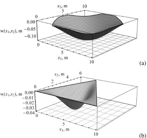
(a)
(b)
Figure 3.Deflectionwof the plates under the action of transverse load: (a) plate with curvilinear boundary; (b) triangular plate, uniform load q=1 MPa (edges are clamped). Here,h=0.1 m,E =200 GPa,ν=0.28. The
image is scaled along the vertical axis for better visibility.
Forq=105sin (πx1\d1) sin (πx2\d2), (7) has the exact solution
we(x1,x2)=
qd4 1d42
π4Dd2 1+d22
2
(d1 = d2 = 10 are the plate sizes). The boundary comprised of various curve pieces was used for
testing purposes. The equation (7) is solved within this domain with corresponding right part and boundary values (9), in which instead of second equation we use Mnw = Mnwe. The numerical
solution of this test problem over a 64×64 grid reaches accuracy of≈10−5(figure 3a) for deflection
value. Let us examine the problem with no known analytical solution. Assume the isotropic triangular plate with vertices (0,0), (10,0), (3,6) is under the uniform transverse loadq=1 MPa. All plate edges are clamped (figure 3b). Results of this numerical experiment are shown in table 3.
5 Conclusion
Only several examples of LSC method calculations for PDE have been demonstrated in this article. This numerical method can be effectively applied to solving a broad variety of practically important problems due to its high versatility.
References
[2] V. I. Isaev and V. P. Shapeev, Comput. Math. and Math. Phys.50, 1758–1770 (2010) [3] W. Cheney,A Course in Approximation Theory(W. Light Brooks, Cole, 2000) 360 pp. [4] J.N. Reddy,Mechanics of Laminated Composite Plates and Shells(CRC Press, 2004) 856 pp. [5] E.I. Grigoluk and T.M. Kulikov, Multilayered Reinforced Shells. Design of Pneumatic Tires
(Mashinostroyenie, Moscow, 1988) 287 pp. [6] N. Pagano, Composite Materials4, 20–34 (1970)
[7] S.K. Golushko, S.V. Idimeshev, and V.P. Shapeev, Computational technologies 19, 5, 24–36 (2014)
[8] S.K. Golushko at al., in MIT-2016, 299–311 (Proceedings, Vrnjacka Banja, Serbia – Budva, 2017)
[9] V.P. Shapeev and V.A Belyaev, Computational technologies21, 5, 95–110 (2016) [10] V.A. Belyaev and V.P. Shapeev, Computational technologies22, 4, 21 (2017)
[11] J.W. Demmel,Applied numerical linear algebra(Philadelphia, PA, USA, 1997) 416 pp. [12] S.P. Timoshenko and S. Woinowsky-Krieger,Theory of plates and shells, 2 ed.(McGraw-Hill,