DOI: 10.1051/epjconf/20122604024 c
Owned by the authors, published by EDP Sciences, 2012
A new probabilistic tool for the determination and optimization of
multiphase equation of state parameters: Application to tin
E. Fraizier
1,a, S. Delattre
2, M. Mougeot
2, Ph. Faure
1, G. Roy
1, and F. Poggi
31CEA, DAM, Valduc, 21120 Is-sur-Tille, France
2LPMA, UFR de Math ´ematiques Paris 7, 75013 Paris, France 3CEA, DAM, Bruy `eres-le-Ch ˆatel, 91297 Arpajon, France
Abstract. A thermodynamically consistent Equation Of State (EOS) was developed to predict and analyse the behaviour of multiphase metals under shock wave loading. Assuming the Mie-Gruneisen hypothesis together with the Birch (for example) formulation, the EOS gives the relation between pressure P, temperature T and atomic volume V. Experimental data (P,V,T) for each phase are provided mainly by X-ray diffraction measurements with diamond anvil cells. In this work, mathematical tools are designed to optimize the determination of the EOS parameters and evaluate uncertainty. The general EOS form isy= fϑ(x)
where y=P, x=(V,T) andϑis the parameter vector to calibrate. Using experimental data (xi, yi), the least square (non-linear)
regression provides an optimal valueϑ∗for the fit parameters. The measurement errors on y and x give biased estimation of
ϑ∗ with the standard method. Assuming centered and known variance laws for the errors, a statistical procedure is proposed
to estimateϑ∗and determine confidence intervals. Thanks to a Bayesian approach it is possible to introduce physical interval knowledge of the parameters in this procedure. Moreover, various EOS fϑ∗formulations are evaluated with a chi-squared type statistical test. The present method is applied on experimental data for multi phase tin (βandγphases and liquid state) in order to provide an optimized multi-phase model. Furthermore, the method is used to design further experimental campaign and to evaluate the gain of new experimental data with the corresponding estimated errors.
1 Introduction
In shock waves experiments on multiphase materials, the diagnostics generally measure only the free surface veloci-ties. The pressureP, specific volumeVand temperatureT need being inferred from hypotheses and calculations. In order to reproduce these velocities and understand the be-haviour of metals under these specific loading conditions, hydrocodes and models (in particular Equation of State -EOS) are developed. In previous works, thermodynami-cally based EOS (Fig. 1) were developed and validated for tin [1–3]. However, input EOS parameters gathered in these works are not always consistent as they originate from various experimental works and/or are determined from different EOS formalisms.
In situ x-ray diffraction experiments in Diamond Anvil Cells (DAC) provide Pressure-Volume-Temperature (P,V,T) data sets that can lead, through an adjustment process, to the determination of an equilibrium EOS [4–9]. This adjustment is classically obtained by a least square regression on the (P,V,T) data with aP= f(V,T) model. With the Mie-Gr¨uneisen hypothesis for each phase the pressure model has the form:
P=Pk(V)+ G0
V0
(T−T0) (1)
The first term Pk(V) describes a reference isothermal (temperature T0) pressure, for instance with the Birch ae-mail:[email protected]
formulation [10]:
Pk(V)=P0+
3 2K0
V V0
−7 3
−
V V0
−5 3
× 1−3
4(4−N0)
V V0
−2 3
−1 (2)
whereG0=Γ0Cv0withCv0is the specific heat constant,Γ0
is the Gr¨uneisen coefficient,K0is the isothermal modulus
andN0is its first pressure derivative. Concerning the units,
T is in Kelvin, P is in GPa, V is in mm3kg−1, andG
0 is
in Jkg−1K−1.N
0 does not have any unit. (T0,P0) defines
the reference condition. It must be noted that experiments under extreme conditions of pressure and temperature are often difficult to perform and therefore data on the material of interest is often scarce, if not lacking. It is interesting, before planning a new experiment in order to increase the accuracy of a multiphase EOS, to evaluate the potential benefit of this experiment, taking into account the foreseen data accuracy and the amount of data to be recorded. For this purpose, some new mathematical tools are developed. These tools should give new information on Birch, Murnaghan [11], Vinet [12] and some others dif-ferent [13–15] formulations for each phase. Furthermore, taking into account the phase transitions determined from experimental data and from the thermodynamically based EOS we plan to optimize each parameter (for each phase). This paper deals with the preliminary steps of this work. The methodology and the mathematical tools principles are detailed. The first results from literature data on tin [5, 6] present the determination of the EOS parameters for
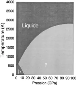
Fig. 1.Multiphase diagram for tin [3].
βandγphases. The maximum uncertainties are used for every (P,V,T) data [5, 6] but, later, the uncertainties should be defined for each point.
2 Methodology description
This work presents mathematical tools designed for op-timizing the determination of the EOS parameters and evaluate the associated errors. This paragraph gives a first overview of the mathematical methodology. The complete mathematical methodology is postponed at the end of the document (see part 5). The general EOS form is Y = fϑ(X) where the output is y = P, the input vector is x=(V,T), andϑis the vector of parameters to be adjusted to best fit the experimental data (xi, yi), i = 1, . . . ,n. This adjustment is classically obtained by a least square regression when the input vector xhas no measurement error and the output quantity y may have measurement error. Indeed, one can prove that the parameters vector vartheta∗
n which minimizes the quadratic misfit, which is the sum of the squared residuals (yi − fϑ(xi))2, is a consistent estimator of ϑ, which means that ϑ∗n tends to the realϑwhenn tends to infinity. The problem is more difficult when the input vector xhas measurement error. In this paper, we propose an estimate ofϑthat takes into account the measurement errors of both xandyand that has a reduced bias compared to the standard least square estimator. This estimatorϑnis theϑwhich minimizesK(ϑ) (see part 5).
From this expression, we can study the estimation error distribution and we can deduce a confidence interval forϑ, which is a direct effect of the measurement errors onxand y. Finally, we study the possibility of taking an a priori knowledge into account. Then we propose a new estimator ofϑ, whose expression is given in part 5.
Moreover, a goodness of fit test is proposed to answer to the question whether the EOS formulation is acceptable or not. A statistical P-value is computed. This quantity follows a uniform law on [0,1] if the EOS formulation is right and is close to 0 if it is not the case.
These mathematical tools are applied to calibrate the studied EOS for tin from available experimental data [5, 6].
Table 1.βphase,a priori.
V0 K0 N0 G0
µ 137230 54.73 5.75 476.7
σ2 105 25 1 2885
Table 2.βphase, parameter estimation using raw data and then with a priori knowledge.
V0 K0 N0 G0
raw data 137204.5 54.37 3.26 482.37
a priori 137218.3 53.98 3.38 482.70
Table 3.βphase, approximate correlation matrix.
V0 K0 N0 G0
V0 1.000 -0.78 0.49 -0.29
K0 -0.78 1.000 -0.90 -0.02
N0 0.49 -0.90 1.000 0.10
G0 -0.29 -0.02 0.10 1.000
3 Application
We study here the EOS given by the Birch model assuming the Mie-Gruneisen hypothesis defined by (1) and (2). The parameters (K0,N0,G0) should be estimated given some
set of experimental data. A R program has been developed
(www.r-project.org) to estimate the parameters using
the proposed methodology. The experimental data corre-spond to non isotherm experiments forβ[5], andγphases [6].
3.1βphase
In [5], theβphase is characterized byn=31 observations where the temperature ranges form 298 to 529 K and the pressure ranges form 0 to 8.5 GPa. The reference state is defined by (P0,T0)=(0,300). The standard deviations for
the measurement errors are σP = 0.13,σV = 125, and σT =2.5.
The a priori knowledge [1] on each parameter is introduced using a Gaussian law N(µ, σ2) defined in Table 1.
The set of parameters is estimated using the raw data without introducing any a priori knowledge on the parameters and then using the a priori. The estimation results are presented in Table 2.
Based on the mathematical analysis, the error distrib-ution on the parameters is computed with the a priori (cf. paragraph 5.4). Table 3 shows the approximate correlation matrix of the estimation errors, using (4) of section 5.5. We observe strong correlations for some parameters as for (K0,N0) and (K0,V0).
The standard deviations areSV0=157.31,SK0=1.80,
SN0 =0.45,SG0 =36.40.
We have conducted a Monte Carlo study to estimate the correlation matrix in parallel (Table 4).
Table 4.Phaseβ, Monte-Carlo correlation matrix, K = 1000 replications.
V0 K0 N0 G0
V0 1.00 -0.77 0.48 -0.27
K0 -0.77 1.00 -0.90 -0.04
N0 0.48 -0.90 1.00 0.11
G0 -0.27 -0.04 0.11 1.00
Table 5.γphase,a priori.
V0 K0 N0 G0
µ 118385 94 4.88 411.6
σ2 1010 25 1 2852
Table 6.γphase, parameter estimation using raw data and with a priori knowledge.
V0 K0 N0 G0
raw data 118248.3 93.23 5.53 564.32 a priori 118264.8 93.04 5.55 554.60
Table 7.γphase, approximate correlation matrix.
V0 K0 N0 G0
V0 1.00 -0.28 -0.15 -0.66
K0 -0.28 1.00 0.50 0.38
N0 -0.15 0.50 1.00 -0.26
G0 -0.66 0.38 -0.26 1.00
to be justified. The P-value to test the physical model equals 0.016. The goodness of the EOS formulation is not rejected at level 1%.
3.2γphase
In [5], theγphase is characterized byn = 38 available observations where the temperature ranges form 298 K to 713 K and the pressure ranges form 4.49 to 16.15 GPa. The reference state is defined by (P0,T0)=(9.40,300).
The standard deviations for the measurement errors are σP=0.24,σV =116, andσT =4.2.
The a priori knowledge on each parameter is intro-duced using a Gaussian lawN(µ, σ2) defined in Table 5.
The set of parameters is estimated using the raw data with-out introducing any a priori knowledge on the parameters and then using the a priori. The estimation results are presented in Table 6.
Table 7 shows the estimated correlation matrix. The respective standard deviation are SV0 = 93.39,
SK0=1.61,SN0 =0.54,SG0=37.24. As for theβphase,
we have conducted a Monte Carlo study to estimate the correlation matrix in parallel (Table 8).
We observe similar correlation matrices computed with the mathematical approach or with Monte-Carlo. The P-value to test the physical model equals 0.027. The good-ness of the EOS formulation is not rejected at level 1%.
Table 8.γ phase, Monte-Carlo correlation matrix,K = 1000 replications.
V0 K0 N0 G0
V0 1.00 -0.28 -0.14 -0.68
K0 -0.28 1.00 0.50 0.34
N0 -0.14 0.50 1.00 -0.25
G0 -0.68 0.34 -0.25 1.00
Table 9.Literature and current work parameters forβtin.
βphase Literature This work: Value Std
V0(mm3.kg−1) 137230 137218 157
K0(GPa) 54.73 53.98 1.8
N0 5.75 3.38 0.45
G0(J.kg−1.K−1) 476.7 482.7 36.4
Table 10.Literature and current work parameters forγtin.
γphase Literature This work: Value Std
V0(mm3kg−1) 118385 118265 93.4
K0(GPa) 94 93.03 1.61
N0 4.88 5.55 0.54
G0(J.kg−1.K−1) 411.6 554.3 37.2
0 5 10 15
115000 120000 125000 130000 135000 140000
P (GPa)
V (mm3.kg-1)
Cavaleri 298K Mabire 298K
This work 298K
Cavaleri 498K Mabire 498K
This work 498K
Fig. 2. Isothermal Birch regression forβtin and experimental data [5].
3.3 Isothermal Birch regressions forβandγphases
The Table 9 summarizes the parameters from literature [1] previously used forβphase and the present results. Then, the isothermal Birch regressions for data tin at 298 K and 498 K are computed and represented on Fig. 2 with the corresponding experimental data from [1].
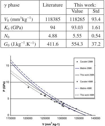
The Table 10 summarizes the parameters from litera-ture [5] previously used forγphase and the present results. Then, the isothermal Birch regressions for γphase at 298 K and 628 K are computed and represented on Fig. 3 with the corresponding experimental data from [6].
0 5 10 15 20
110000 115000 120000 125000 130000 135000 140000
P (G
Pa)
V (mm3.kg-1)
Plymate 298K
Mabire 298K
This work 298K
Plymate 623K
Mabire 623K
This work 623K
Fig. 3. Isothermal Birch regression forγtin and experimental data [6].
data [5, 6] and Birch formulation whereas the literature parameters integrate several experimental data.
4 Conclusion, benefits and perspectives
A first step of a new tool development to determine the multiphase EOS parameters is reached. The resulting parameters enable to compute isothermal Birch regression in good agreement with experimental data. We can now integrate more experimental data and test different Pk(V) formulations. Furthermore, the literature data can be used as an a priori on data. This tool will be used to determine the benefits of new experimental campaign or new diag-nostics including the uncertainties. The matrix correlation of theV0,K0,N0andG0parameters is estimated and gives
further information. A Monte Carlo study, conducted in parallel, shows similar results for this matrix and vali-dates our approach. Furthermore, a P-value quantifies the goodness of physical model. Then, this new tool gives the opportunity to test different Pk(V) formulations. The last perspective is to optimize every parameters of each phase, taking into account the experimental transitions and our thermodynamically based EOS model.
5 Annex: Mathematical results
5.1 Statistical model
Consider two physical variablesx=(x1, . . . ,xd)∈Rdand y∈Rlinked by the following equationy=φ(x) whereφis a function fromRdtoR. An equation of state formulation is defined by a family of functions onRd:
fϑ:Rd→R, ϑ∈Θ⊂Rk
where ϑ = (ϑ1, ϑ2, . . . , ϑk) corresponds to the physical parameters. The EOS formulation is relevant ifϕis mostly equal to fϑ∗ for a given value ϑ∗ ∈ Θ. Considering n physical points (x1, y1), . . . ,(xn, yn), an approximation of ϑ∗ is given by ϑ∗
n satisfying κ(ϑ∗n) = minϑΘκ(ϑ) where κ(ϑ) = n−1 n
i=1(yi− fϑ(xi))2. If the EOS formulation is relevant one can expectϑ∗n =ϑ∗forn≥k, as in the Birch formulation for instance.
The physical points (xi, yi) are only known through ex-perimental measurements (Xi,Yi). The measurement errors
are modeled as follows: – Xi∼ Nxi,σ2
X) is a Gaussian random vector with mean
xi and covariance matrix σ2
X (typically a diagonal
matrix). – Yi∼ N(yi, σ2Y).
– The random vectorsXi,Yi, 1≤i ≤nare supposed to be independent.
5.2 Estimation
The least square estimation ˆϑofϑ∗is defined byK( ˆϑ)= minϑ∈ΘK(ϑ) where K(ϑ) = n−1 n
i=1
Yi − fϑ(Xi) 2
.A1:
The function(ϑ,x) → fϑ(x)is supposed to be sufficiently smooth.Θis a compact set. There exists a uniqueϑ∗n ∈Θ such thatκ(ϑ∗n)=minϑ∈ϑκ(ϑ).
Theorem 1 AssumeA1. As σ2X → 0 and σ2Y → 0, the distance betweenϑˆandϑ∗ntends to0in probability:
f or allε >0, Pϑˆ−ϑ∗n> ε
→0.
5.3 Estimation error distribution
Notation: For ϑ = (ϑ1, . . . , ϑk) and x = (x1, . . . ,xd), define the column vectors
˙ fϑ(x)=
∂ ∂ϑi
fϑ(x)
1≤i≤k
, fϑ(x)= ∂
∂xi fϑ(x)
1≤i≤d ,
thek×kmatrix ˙ fϑ(x)=
∂2 ∂ϑi∂ϑj
fϑ(x)
1≤i,j≤k
and thed×kmatrix ˙ fϑ(x)=
∂2
∂xi∂ϑj fϑ(x)
1≤i≤d,1≤j≤k .
IfMis a matrix,Mdenotes its transpose. We introduce the assumption:
A2: A1 holds true and ϑ∗n belongs to the interior of Θ. Moreover the Hessian matrix ofκatϑ∗nis positive definite. Note that the Hessian matrix ofκatϑ∗nis equal to
Λ=n−1
n
i=1
˙ fϑ∗
n(xi) ˙fϑ∗n(xi) −n−1
n
i=1
(yi−fϑ∗n(xi)) ˙fϑ∗n(xi).
Theorem 2 AssumeA2. Asσ2X→0andσ2Y→0, ˆ
ϑ−ϑ∗ n=n−1
/2Λ−1Γ1/2Z+O||σ2
X||
(3) where:
– σ2Xdenotes the largest eigenvalue ofσ2X
– Γis the k×k matrix
1 n
n
i=1
σ2
Yfϑ˙∗n(xi) ˙fϑ∗n(xi)
+M(y
i,xi, ϑ∗n)σ2X ×M(yi,xi, ϑ∗n)
withM(yi,xi, ϑ∗n)=(yi−fϑ∗n(xi)) ˙fϑn∗(xi)−fϑ˙∗n(xi)fϑ∗n(xi). When the second term of (3) is negligible, the first term provides the probability distribution of the estimation error, namelyN(0,Σ/n) withΣ=Λ−1ΓΛ−1, which order of magnitude is less thann−1/2(||σ2
X||1
/2+σ
Y).
Remark 1 For a large numbernof observations and when σ2
Xis known, the standard least square contrastK(ϑ) can
be successfully replaced by 1
n n
i=1
Yi− fϑ(Xi) 2−
fϑ(Xi)σ2Xfϑ(Xi)
which provides an estimation ofϑ∗n with a reduced bias, still of orderO(||σ2
X||), when fϑ(x) is a bilinear function of
ϑandx.
5.4 Confidence interval
We construct confidence intervals for the componentϑ∗n,i ofϑ∗n and more generally foruϑ∗n whereuis a vector of Rk
. From Theorem 2, ifuΣu ||σ2X||then n1/2(uϑˆn−uϑ∗n)σN(0,uΣu).
Moreover uΣu can be approximated by uΣˆu where ˆ
Σ is the empirical version of Σ, replacing (xi, yi, ϑ∗n) by (Xi,Yi,ϑ). Finally we obtain thatˆ
n1/2(uϑˆn−uϑ∗n) uΣˆu
1/2∼ N(0,1).
This gives directly confidence intervals foruϑˆn.
5.5 Use of a priori knowledge
We propose here a method which takes benefit of a pre-vious estimation ofϑ∗n. Assume that we have some infor-mation on the firstpcomponents ofϑ∗n,1, . . . , ϑ∗n,pofϑ∗n= (ϑ∗
n,1, ϑ∗n,2, . . . , ϑ∗n,k) (1 ≤ p ≤ k), that is we observe a p-dimensional random vector ˆτ, independent of ˆϑ, following the lawN(τ∗n,Σ˜) whereτ∗n=(ϑn∗,1, ϑ∗n,2, . . . , ϑ∗n,p) and ˜Σis a givenp×pcovariance matrix (positive definite).
ˆ
ϑhas been previously computed and satisfy ˆ
ϑ−ϑ∗
n∼ N(0,Σˆ/n).
The new estimator ˜ϑnwe can compute is the “best” linear combination of ˆϑand ˆτ:
˜
ϑ=(nΣˆ−1+Γ˜)−1
nΣˆ−1ϑˆn+
˜
Σ−1
ˆ τ 0
where ˜Γ =
˜
Σ−10
0 0
is ak×kmatrix. The estimator ˜ϑis approximatively Gaussian, with non bias and covariance matrix equal to
(nΣˆ−1 +Γ˜)−1. (4) Note that ˜ϑ is always as good as ˆϑ since (nΣˆ−1 + ˜
Γ)−1≤Σˆ/n.
5.6 Feedback and test on the physical model
Can we detect whether the EOS formulation is good or not? In other words are the yi − fϑ∗n(xi), 1 ≤ i ≤ n, significantly not equal to zero?
Introduce the log-likelihood contrast: forϑ∈Θandn vectorsξ1, . . . , ξn∈Rdset
L(ϑ, ξ1, . . . , ξn)= n
i=1
Yi−fϑ(ξi)2 σ2
Y
+(Xi−ξi)(σ2X)−
1(Xi−ξ
i)
.
A3:A1 holds.ϑ∗n belongs to the interior ofϑ. Moreover yi= fϑ∗n(xi)for i=1, . . . ,n.
Theorem 3 AssumeA3. As σ2Y → 0 and σ2X → 0, the
distribution of the random variable
D= min ϑ,ξ1,...,ξn
L(ϑ, ξ1, . . . , ξn)
converges to the chi-square distribution with n−k degrees of freedom.
Therefore, iftdenotes the computed value ofD, the proba-bilityP(χ2
n−k >t) is an approximateP-value for testing if the EOS formulation is relevant (the null hypothesis here).
References
1. C. Mabire, Ph.D. thesis, Poitiers Univ. France (1999) 2. C. Mabire, P. Hereil, Shock Compression of
Con-densed Matter (2000)
3. F. Buy, C. Voltz, F. Llorca, Shock Compression of Condensed Matter (2005)
4. M. Liu, L. Liu, High Temp. - High Pressures 18, 78 (1986)
5. M. Cavaleri, T. Plymate, J. Stout, J. Phys. Chem. Solids8(49), 945 (1988)
6. T. Plymate, J. Stout, C. M.E., J. Phys. Chem. Solids 49(11) (1988)
7. N. Rambert, P. Faure, B. Sitaud, 40th European High-Pressure Meeting, Edimbourg (2002)
8. R.J. Angel, in High-pressure and high-temperature crystal chemistry(2000), Vol. 41, pp. 35–60, r. hazen and r downs editors edn.
10. F. Birch, J. Geophys. Res.83, 1257 (1978)
11. F.D. Murnaghan, Finite Deformation of an Elastic Solid(Wiley, New York, 1951)
12. P. Vinet et al, Phys. Rev. B35(1986)
13. P. Bose Roy, J. Bose Roy, J. Phys: Condens. Matter17 (2005)
14. P. Bose Roy, J. Bose Roy, J. Phys: Condens. Matter18 (2006)
![Fig. 3. Isothermal Birch regression for γ tin and experimentaldata [6].](https://thumb-us.123doks.com/thumbv2/123dok_us/8082192.1348625/4.595.85.250.68.193/fig-isothermal-birch-regression-g-tin-experimentaldata.webp)
