144
possible to design range surveys
to estimate pellet group numbers
and to collect pellet group sam-
ples. Cellulose assay of pellet
groups combined with a knowl-
edge of deer food habits upon a
particular range would seem to
offer a potentially useful tech-
nique to estimate forage utiliza-
tion by deer.
LITERATURE CITED
ASSOCIATION OF OFFICIAL AGRICUL- TURAL CHEMISTS (AOAC). 1960.
SHORT AND REMMENGA
Official Manual of Analysis. 9th Ed. Washington, D.C. XX + 832 PP.
BARNETT, A. J. G. AND R. L. REID. 1961. Reactions in the rumen. Edward Arnold (Publishers) Ltd., London. VIII + 252 pp.
DAVIS, R. B. 1952. The use of rumen contents data in a study of deer- cattle competition and “animal equivalence.” Trans. N. Am. Wildl. Conf. 1’7: 448-458.
SALSBURY, R. L., C. K. SMITH, AND C. F. HUFFMAN. 1956. The effect of high levels of cobalt on the in
vitro digestion of cellulose by ru- men microorganisms. J. Anim. Sci. 15: 863-868.
SHORT, H. L. 1963. Rumen fermenta- tions and energy relationships in white-tailed deer. J. Wildl. Man- age. 27: 184-195.
SMITH, A. D., R. B. TURNER, AND G. A. HARRIS. 1956. The apparent di- gestibility of lignin by mule deer. J. Range Manage. 9: 142-145. WISE, L. E., AND E. C. JAHN: editors.
1952. Wood Chemistry. Reinhold Publ. Corp. New York. Vols. 1 and 2.
Prediction of Weight Composition from
Point Samples on Clipped Herbage’
HAROLD F. HEADY AND GEORGE M. VAN DYNE2 Professor of Forestry (Range Management) and Re- search Nutritionist, University of California, Berkeley and Davis.
Highlight
Percentage botanical composition by weight can be estimated from composition determined with the, laboratory point method, if differ- ences among species, seasons of growth, and botanical composition are taken info account.
Weight of herbage is an attri-
bute of individual plants and
plant communities that has been
measured since the beginning of
intensive pasture
and range
studies. Many procedural varia-
tions in weight sampling have
been suggested
(Brown, 1954;
U.S. Forest Service, 1958). While
total herbage
weight
is fre-
quently reported, percentage
species composition on a weight
basis is seldom given because
hand separation is time consum-
ing and, therefore,
expensive.
Pechanec and Pickford
(1937)
suggested weighing the whole
1
Partial support from USDA West- ern Regional Research Project W-34 and NIH Grant FR-00009 is gratefully acknowledged.2 Present address: Radiation Ecology Section, Health Physics Division, Oak Ridge National Laboratory, Oak Ridge, Tennessee.
sample and estimating the parts.
Although estimates can be cor-
rected and the estimators trained
by double sampling techniques
(Wilm et al., 1944), ocular esti-
mates have personal bias.
Field point sampling of foliage
and basal cover is frequently
used to determine percentage
species composition. Recently,
laboratory point sampling has
been employed to determine
composition of forage samples
taken from f istulated
animals
(Van Dyne and Torell, 1964). Re-
ports are scarce of attempts to
estimate percentage weight com-
position with point sampling.
Heady and Tore11 (1959) pre-
sented graphs which suggested
that field points, laboratory
points, and weights by hand sep-
aration gave similar species com-
positions. Harker, et al. (1964)
found that percentage species
composition by the microscopic
point method gave a satisfactory
estimate of composition on a dry
weight basis in controlled mix-
tures of a coarse grass and sweet
potato vines.
Field time is more limited
than laboratory time in many
range investigations.
Propor-
tional species weights in the
field and in animal diets have
more meaning in certain studies
than proportions based on cover.
Therefore, techniques for rapid
and accurate estimating
of
weight composition are needed.
The purpose of this study was
to develop and test equations
which predict percent weight
composition (Y) from percent
point composition
(X) .
Several
questions were examined in ana-
lyzing point-weight
relation-
ships: (1) Is transformation of
the variates necessary? (2) Are
prediction equations
adjusted
through the origin superior to
those not through the origin?
(3) Are separate prediction
equations needed for individual
species or can they be grouped
conveniently without losing pre-
cision? (4) Can prediction equa-
tions developed for immature
plants be used for mature
plants? (5) Does variation in
vegetational composition affect
the usefulness
of prediction
equations?
(Table 1). Full
description of
the treatments and results were
discussed by Heady and Tore11
(1959). The resident annual and
soft chess enclosures were high-
est in grass because mulch was
left in place in the former and
only partially removed in the
latter. Soft chess
(Bromus mollisL.) was seeded in the soft chess
enclosure. Where all mulch was
removed,
broadleaf
filaree
(Erodium botrys
Bertol.) was of
greatest percent weight. Seeding
bur clover
(Medicago hispidaGaertn.) and removing part of
the mulch resulted in vegetation
with a large clover portion and
the least filaree. Thus, the point-
weight relationships
in this
paper were developed for mixed
annual vegetation in which soft
chess, filaree, and bur clover
contributed 91 to 96 percent of
the total weight. Wider varia-
tions among these species than is
shown in Table 1 occur in the
California annual type between
locations and between
years
(Heady, 1961).
Sampling. -Ten plots each one ft3 were clipped in each enclosure on five dates in 1958: February 1, March 6, April 2, May 2, and July 8. These dates covered essentially the whole growing season in the annual grass type. The ten clipped samples for each date were composited and thoroughly mixed. From each com- posite sample, ten sub-samples were analyzed with 50 points that were taken with a binocular microscope technique described by Heady and
Tore11 (1959) and illustrated by
Table 1. Percentage botanical com- position by weight in four en- closures averaged for five sam- pling dates between February and July, 1959.
All1 B. E. M.
Enclosure gr. mol. bot. his.
Resident
annual 42 34 57 <l
Soft chess 35 31 54 10
Filaree 22 20 68 7
Bur clover 29 26 34 37
1 All gr. = all grasses; B. mol. =
Bromus mollis; E. bot.=Erodium
botrys; M. his.=Medicago hispida.
The hypothesis that Y, = 0 when X1 = 0, i.e., that zero points equal zero weight, was accepted because
~2 values were somewhat higher
when the regression lines were ad- justed to pass through the origin (Table 3). In testing this hypothe- sis, the sample size was 538 for all grasses, 422 for all forbs, 136 for grasses in July, and 113 for forbs
in July. The data contained 149
items of Y, = >0 but X1 = 0 and 18 items of Y, = 0 but X1 = >O. Over 70 percent of these values greater than zero were less than 2
percent. They are small errors in
double sampling that bias the results
positively because neither percent
points nor weights of less than zero
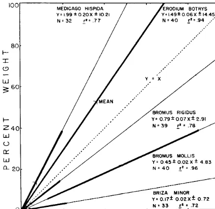
Individual species varied widely
in the ratio of weight to points and in the predictive equations (Figure 1). The dotted lines, Y = X, repre- sents weight composition estimated by point composition on a 1: 1 ratio. Generally, all the forbs were above this ratio and all grasses below it. Full regression equations are shown in Figure 1, including the standard error of regression coefficient, stan- dard error of estimate, sample size
(N) , and ~2 values. The heavy part of each regression line shows the mean percent points f three stan- dard deviations.
. Soft chess composed 48 percent of
the point composition in July over all plots and filaree 36 percent. The predictive equations for these two species on each of the five dates was
approximately equal to the equa-
tions for all grasses and for all forbs on the corresponding dates. For ex- ample, the average slope of the re- gression line for all grasses in July was 0.46 and all forbs 1.50. This suggests that forbs and grasses can be grouped separately if objectives permit.
Table 2. Relafionship of percent weight (Y) fo percent points (X) with four types of transformations.
Standard error
Transformation Equation of estimate r2 .lOO
qx+1, b3oy Y= 0.32+ 0.17X 0.16 83
Arcsin (X+1), LogroY = 0.67+ 1.67X 0.18 77
-~
vx+1, Y =-9.96+ 5.91X 6.82 76
Arcsin (X-l-l), Y = 1.25+60.8X 6.35 79
X, Y = 1.21+ 0.66X 6.19 81
Harker et al. (1964). Point analyses were made on fresh herbage as it came from the field in order to minimize shattering. Each subsample
was hand separated into species,
dried, and weighed.
Resulis Equation Selection
Several types of transformations were made to determine whether
the regression lines were linear,
curved, or unduly influenced by per- centages. Typical results are shown for grasses clipped in February with a sample size of 81 (Table 2).
Arcsin transformations to correct
for percentage distributions gave
lesser ~2 values than those calculated
from percentages. Square root and
logarithmic transformations indicate
that linear relationships exist be-
tween percentage points and per- centage weight because the r2 values were only slightly larger or smaller
than the coefficient when both X
and Y were on a linear scale. On the other hand, the standard error of estimate of the linear regression line is somewhat larger than the
others. Little is gained by these
transformations so percentages as
computed from original data were used.
Table 3. The relationship (r2.100) between perceti points (X) and percent weight (Y) for equations through or noi through the origin.
Not
Through Through
Data Group Origin Origin
All grasses 85 92
All forbs 88 95
Grasses in July 89 93
Forbs in July 86 92
could occur. Adjusting the regres- sion lines to pass through the origin corrects for this bias. Between 92 and 95 percent of the variation in percentage weight is accounted for in the variation of percentage points
for equations through the origin
(Table 3).
146
HEADY AND VAN DYNE
80. t- I a -
60 80 POINTS
FIGURE 1. Regression of percent weight on percent points
for five species over all plots in July. Mean per- centage point composition is shown on each regression line.
The equations for all grasses and
forbs were developed from indi-
vidual species data in each sample rather than on the sums of grasses and forbs in the samples. N would have been 200 in the latter calcula- tions. If equations were developed
with sums, false confidence is ob-
tained because sampling errors tend to be canceling and variance reduced in summation of percentages.
Sets of 50 points were considered a sample in contrast to the usually reported 100 to 400 points. Relatively small standard errors indicate that
cornpositing of material and sub-
sampling can be used to reduce
sample size if knowledge of field
variation is not essential.
The range in slope from 0.17. for little quaking grass (Briza minor L.) to 1.99 for bur clover is caused by difference in plant structure. Little quaking grass has a large open in- florescence with fine branches that weigh less per point than the other
species. Ripgut (Bromus rigidus
Roth.) is a coarser plant than soft
chess. In July, after many forb
leaves had shattered, the stems of bur clover weighed more per point than those of filaree. Examples of
slopes or weight:point ratios for
other species are 0.32 for nitgrass
(Gastridium ventricosum (Govan)
Schinz and Thell.), 0.48 for galium
EO- t- I c3 - W
20 PERCE4:T
60 POINT:’
FIGURE 2. Regression of percent weight on percent points for grasses and forbs at five periods during the grow- ing season.
(Galium parisiense L.), and 1.00 for
turkey mullein (Eremocarpus seti-
gerus Benth.) .
Stage of Mafurify
Until approximately the first of
April, plants in the California an- nual type are short with little stem
material. Stem elongation occurs
and flower parts emerge as soon as temperatures rise. In the year the samples were taken, plants were short during the first three sampling periods, approaching maturity at the May sampling, and over a month past maturity in July. Within grasses and forbs, slopes of the prediction equations for February, March, and
April were essentially the same
(Figure 2). In May, forbs weighed more per point and grasses less than earlier in the season. The trend continued in July.
High predictive value of these
equations is indicated by narrow
confidence limits on the predicted
percentage weights at the mean of percentage points (Table 4). At the extremes of low and high percent- age points the predictive values are less. The confidence limits for the different lines overlap at point per- centages below 6 to 13, indicating a minimum level where difference be-
Data in Table 4 apply to the regres- sion lines in Figure 2.
Predicted percentage weights were less for grasses than the percentage points and the reverse was true for
forbs (Table 4). That is, grasses
weigh less per point than do forbs,
or assuming constant density of
plant material, there is greater
cross-sectional area per point for
Table 4. Predicfed percent weighf (q), wifh confidence limifs (C.L.) af ihe 95% level, for all grasses and forbs af five dates, (a) c&u- la&l af fhe mean percentage point
composifion (X5 Standard error)
and (b) confidence limits af fhe
mean point composifion + three
standard deviations.
(a) (b)
P+_C.L. -I-C.L. %S.E.
GRASSES
Feb. 18kO.25 4.31 26k2.1
March 1520.14 3.78 22k2.3
April llkO.16 2.91 17-1-1.8
May lleO.12 2.48 20+2.2
July 8+0.08 1.88 17+1.9
FORBS
Feb. 33kO.31 5.63 26k2.3
March 36kO.29 5.27 28+2.3
April 3220.08 2.30 25k2.0
May 3020.30 5.28 21k1.9
July 23kO.32 6.15 15k1.7
forbs than for grasses. These differ- ences were maintained through the growing season and became accen-
tuated because more forb leaves
shattered than grass leaves.
The comparisons thus far made
were on a basis of point sampling of clipped material with the binocu-
lar microscope. Percentage foliage
cover of grasses, on a basis of field point sampling, was lowest in March
and highest in July (Table 5).
Heights of the field hits were mea- sured with the apparatus described by Heady and Rader (1958). Aver- age height and average weight per square foot gradually increased until April, reached a peak in May after a short rapid growth period, and de- clined as the dry season progressed, agreeing with earlier findings (Rat- liff and Heady, 1962).
Ratios of percentage weights to
percentage points decreased more
for grasses in the field than was
shown in the laboratory sampling,
although the two trends are similar.
Percentage cover of grasses in-
creased but percentage weight de-
creased, thus accounting for the
lower ratios. Forbs showed an in- crease in weight per point in the field over results in the laboratory.
As relative forb cover decreased
relative weight increased.
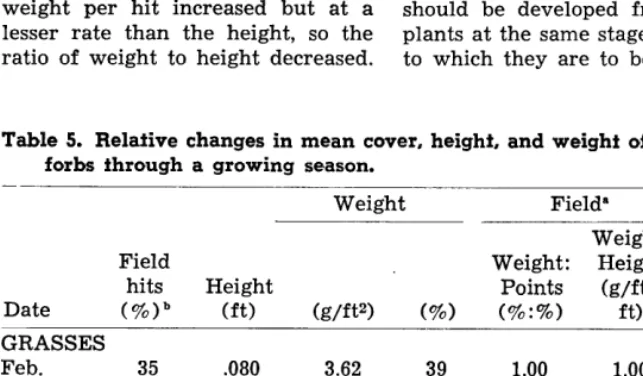
As all plants grew taller, the weight per hit increased but at a lesser rate than the height, so the ratio of weight to height decreased.
Grasses showed this relationship
more than forbs. Even though
grasses were always taller than the forbs, the latter were always heavier per point and became increasingly heavier with growth. Observations agree with the data in suggesting that stems and fruiting parts of the forbs increased in coarseness more than the same parts of grasses. Evi- dently the effect of shading on the forbs by grasses did not cause the forbs to lengthen and develop thin stems.
Decrease in weight and height from May to July was due to normal shattering of leaves and inflores- cences and to the actions of small animals. The enclosures were un- grazed by livestock. Decrease in the ratio of weight to height in grasses and an increase in forbs from May to July is because of more weight loss in shattering of grasses than of
forbs. This is probably because of
the more complete shattering of in- florescences in the grasses.
These data suggest that each hit has a certain weight value that is different for grasses and forbs. The values change through the growing season, especially during the periods of rapid growth and shattering after plant maturity. For equations to be
most useful in predicting percent
weight from percent points they should be developed from data on plants at the same stage of maturity to which they are to be applied.
Table 5. Relative changes in mean cover, height, and weight of grasses and forbs through a growing season.
-
Weight Field” Lab
Weight:
Field Weight: Height Weight:
hits Height Points (g/ft? Points
Date (%)” (ft) (g/ft? (%I (%:%) f t) (%:%)
GRASSES
Feb. 35 .080 3.62 39 1.00 1.00 1.00
March 32 .lOl 4.29 36 1.01 0.94 0.99
April 34 .136 4.53 33 0.87 0.74 0.99
May 35 .415 11.75 32 0.82 0.63 0.80
July 42 .292 6.10 27 0.58 0.46 0.66
FORBS
Feb. 65 .050 5.55 61 1.00 1.00 1.00
March 68 .076 7.74 64 1.00 0.92 1.00
April 66 .108 9.17 67 1.08 0.76 1.01
May 65 .310 25.22 68 1.12 0.73 1.12
July 58 .188 16.61 73 1.34 0.80 1.18
* All ratios are adjusted to those of February equalling 1.00. b Percentage field hits are based on 1600 points at each date.
Species Composition
As indicated earlier, the four en- closures had different species com- position at the time of sampling (Table 1). Averaged over all dates, ratios of percentage weight to per-
centage points increase for both
forbs and grasses as the proportion of grass in the stand increased (Fig- ure 3). The lowest weight per point occurred on the filaree plot and the highest on the resident annual plot. Forbs on the forb plots had thinner plant parts and less weight per point on the average than forbs on the
grass plots. Conversely, grasses on
the grass plots had more weight per point than grasses on the forb plots. These differences were not consis-
tently significant above approxi-
mately 20 percent composition, be- low which no significant differences were found.
Change in plant form may be the result of more lower leaves dying in relatively pure grass stands. There- fore, the proportion of stems in the
total herbage and the average
weight per point would be greater than in mixed stands. Such an ex-
planation fits the relationships of
grasses in the plots but not the forbs.
Forbs may react differently by
prrowing taller with thinner stems. Whatever the cause, weight to point
ratios change with differences in
composition, but these changes are of less magnitude than those asso- ciated with stage of maturity and species.
Summary
Regression analyses show that
nercentage botanical composition
by weight can be estimated from
composition determined with the
laboratory point method. This
conclusion is based on point
sampling with a binocular micro-
scope of clipped herbage and
hand separation of the same ma-
terial.
Satisfactory results were ob-
tained by analysis of the per-
centage data, on a linear basis
through the origin,
without
transformation of the variates.
148
100
t- *O I (3 - w 3 6o
I- z 40
W 0 LT W
a 20
0
HEADY AND VAN DYNE
- - RESIDENT ANNUAL 96 -._ SOFT CHESS
---- - BUR CLOVER - FILAREE
20 60 100
P E R C E4i T
POI
NT s””
FIGURE 3. Change in ratio of percent weight to percent points for forbs and grasses from plots of different species composition.
1.00 to 1.99. Prediction equations for all grasses combined and all forbs combined were similar to the equations for the dominant species of each group at each sampling period.
Ratios of weight to points changed during the growing sea- son because of changing thick- ness of plant parts, shattering, and varying proportions of plant parts. With maturity, forbs be- came heavier and grasses lighter per point, whether measured in
the field or laboratory. In the field grasses increased while forbs decreased in herbage cover and grasses increased in height more than forbs. Weight to height ratios decreased in both forbs and grasses but more so in the grasses.
Regression of percent weight on percent points varied with species composition, although not as much as among species and through the growing season. Percentage weight composition
can be estimated satisfactorily from laboratory point analysis, if differences among species, sea- sons of growth, and botanical composition are taken into ac- count.
LITERATURE CITED
BROWN, DOROTHY. 1954. Methods of surveying and measuring vegeta- tion. Commonwealth Bur. Pastures and Field Crops. Bul. 42. 223 pp. HARKER, K. W., D. T. TORELL, AND G. M. VAN DYNE. 1964. Botanical ex- amination of forage from esopha- geal fistulas in cattle. J. Anim. Sci. 23: 465-469.
HEADY, H. F. 1961. Continuous vs.
specialized grazing systems: A re- view and application to the Cali- fornia annual type. J. Range Man- age. 14: 182-193.
HEADY, H. F. AND L. RADER. 1958.
Modifications of the point frame.
J. Range Manage. 11: 96-97. HEADY, H. F. AND D. T. TORELL. 1959.
Forage preference exhibited by
sheep with esophageal fistulas. J. Range Manage. 12: 28-34.
PECHANEC, J. F. AND G. D. PICKFORD.
1937. A weight estimate method for determination of range or pas-
ture production. J. Amer. Sot.
Agron. 29: 894-904.
RATLIFF, R. D. AND H. F. HEADY. 1962.
Seasonal changes in herbage
weight in an annual grass commu- nity. J. Range Manage. 15: 146-149. U. S. FOREST SERVICE. 1959. Tech - niques and methods of measuring understory vegetation. S o u t h e r n
and Southeastern Forest Expt.
Stations. 174 pp.
VAN DYNE, G. M. AND D. T. TORELL. 1964. Development and use of the
esophageal fistula: A review. J.
Range Manage. 17: 7-19.
WILM, H. G., D. F. COSTELLO AND G.
E. KLIPPLE. 1944. Estimating forage
yield by the double-sampling
method. J. Amer. Sot. Agron.