Abstract—The University of Florida is taking a multidisciplinary approach to fuse the data between 3D vision sensors and radiological sensors in hopes of creating a system capable of not only detecting the presence of a radiological threat, but also tracking it. The key to developing such a vision-aided radiological detection system, lies in the count rate being inversely dependent on the square of the distance. Presented in this paper are the results of the calibration algorithm used to predict the location of the radiological detectors based on 3D distance from the source to the detector (vision data) and the detectors count rate (radiological data). Also presented are the results of two correlation methods used to explore source tracking.
I. INTRODUCTION
his project combines 3D vision sensors and radiological detectors in hopes to more efficiently and effectively locate potential nuclear threats in dynamic environments such as airports and package and mailing facilities. Any radioactive material may pose a health threat and could lead to harm if transported undetected and/or used in radiation dispersion devices (RDDs). Special nuclear material (SNM) is also a major concern as it can potentially be used in nuclear weapons [1]. Current systems such as portal monitors and distributed sensor networks approach this issue [2] [3]. However, the system discussed in this paper would not only be able to determine the presence of a nuclear threat, it would be able to track it; thus, allowing less disturbance of commerce and more accurate secondary inspector response.
Combining radiological sensors with vision sensors will help to see potential occlusions, suspicious persons or items, and determine if there is a cause for concern. It is possible to combine radiological sensors and vision sensors through data fusion. The ability to correlate a time dependent signal of a moving source is the key to fusing the two systems. Fig. 1 shows the conceptual idea of conjoining the time dependent data sets of the two types of sensors. The concept is based on the radiological count rate being inversely dependent on the square of the distance.
June 1, 2017. This material is based upon work supported by the U.S. Department of Homeland Security under Grant Award Number, 2014-DN-077-ARI083-01. The views and conclusions contained in this document are those of the authors and should not be interpreted as necessarily representing the official
Fig. 1. Tracking scenarios and the principle of the overlapping distance/time domain between the radiological and visual sensor. The scales will be arbitrary but the data trends will be highly correlated.
Ideally, the choice of 3D vision sensors, radiological detectors and fusion algorithms can be flexible for implementation purposes. Due to their long range in air and their ability to travel through some shielding and visually opaque materials, gamma-rays and neutrons are the most useful quanta to detect compared to beta and alpha particles. Detectors with the capability of detecting both Gamma rays and neutrons and then differentiating between the two with pulse shape discrimination methods may be advantageous. A wide range of radiological detectors consisting of EJ-309 liquid scintillators, Na-I, and He-3 have been explored.
Vision sensors such as the Microsoft Kinect and the Velodyne HDL-32E LiDAR have been explored for this research. The Kinect uses an infrared (IR) emitter, which emits infrared light beams, and a depth sensor, which reads the IR beams reflected back to the sensor. The reflected beams are converted into depth information measuring the distance between an object and the sensor [4]. The Velodyne uses Light Detection and Ranging (LiDAR) technology, which measures distances using Time of Flight (TOF) and short laser pulses. Massachusetts Institute of Technology is currently working on depth sensing with polarization cues, which will drastically improve cheap 3D imaging sensors [5]. This paper will only cover the results using the Velodyne HDL-32E and the EJ-309 liquid scintillators. However, two correlation algorithms and their results will be discussed.
Before taking dynamic measurements in a room, the room
policies, either expressed or implied, of the U.S. Department of Homeland Security.
Kelsey Stadnikia is with the University of Florida, Gainesville, FL 32606 USA (e-mail: [email protected]).
Data-Fusion for a Vision-Aided Radiological
Detection System: Sensor dependence and
Source Tracking
Kelsey Stadnikia, Allan Martin, Kristofer Henderson, Sanjeev Koppal, Andreas Enqvist
must be calibrated. To do this, a calibration algorithm is used to predict the location of the radiological detectors based on the 3D distance from the source to the detector (vision data) and the detectors count rate (radiological data). Thus, count rate can be correlated to movement in three dimensions.
II. METHODS AND MEASUREMENTS
An experimental setup utilizes EJ-309 Liquid Scintillator detectors and an HDL-32E LiDAR. Calibration experiments are
used to determine a detector “pseudo-location” and involve
several static measurements. The “pseudo-location” is where
the data fits best and takes into account room and detector dependencies. Correlation experiments involve the potential
use of this discovered “pseudo location” and dynamic
measurements.
A. Calibration
For calibration, a Cf-252 source is placed in a camera calibration target resembling a checkerboard and is measured in 27 static locations arranged in a 3x3x3 cube. One EJ-309 detector is setup to be collocated with the HDL-32E while another is setup in an offset location. Fig. 2 shows a schematic of this setup for nine individual experiments.
Fig. 2. Top-down view of the room in the x and y directions. The yellow star represents the known location of the co-located detector. Red dots represent the 27 source locations. Orange circles represent the manually measured offset detector locations. Blue blocks represent fixed lab furniture that may cause radiation scattering. Not to scale.
The calibration algorithm is based on (1).
𝑅𝑅 𝑅 𝑅𝑅0𝜆𝜆𝜆𝜆𝜆𝜆𝜆√𝐶𝐶 (1)
R represents the 3D distance from the source to the offset detector, whereas, R’ represents the distance from the source to the collocated detector. C is the count rate collected by the collocated detector and λ0 is a scaling factor used to account for source strength. The algorithm begins by determining λ(R’) using the count rate collected by the collocated radiological detector and the 3D distance from the collocated radiological detector to the source as determined by the vision sensor. This function is determined to be a second order polynomial fit to the data which can be seen in Fig. 3.
Fig. 3. Second order polynomial fit to combined data, gamma-ray only data, and neutron only data.
The parameter λ0 is determined by exploring a wide range of values. The algorithm then generates spherical shells of a given thickness and radius R at each individual source location. Where the majority of these spherical shells overlap is said to
be the “pseudo-location”. The spherical shell generation and
progression can be seen in Fig. 4. The point where the most spherical shells overlap then determines the number of voxels overlapped and averages the voxels to output one location with x, y, and z coordinates. The optimal λ0 value is chosen where the most spherical shells overlap and then where the most voxels are covered by the overlaps.
Fig. 4. Horizontal (2D) slices in the x-y plane illustrating the overlapping spherical shells used in the algorithm at various heights in the z directions (top-left: -213 cm, top-right: -129 cm, bottom-(top-left: -72 cm and bottom-right: -12 cm). x, y, z directions correspond to left-right, forward-backward and up-down directions for the vision sensor view respectively.
The location determined by the algorithm now represents the
“pseudo-location” where the data works best. Thus, allowing
the accuracy of the predicted sensor location to presumably be ignored. Further analysis will determine the eligibility of this approach. Once the room is calibrated, dynamic source tracking can take place. Results of the calibration algorithm are done using hand measured location data, as well as, vision sensor location data.
B. Correlation
Numerous measurement scenarios comprising of two to three people walking in a room where one of the persons is carrying a source in a backpack have been taken. Choreographed walking patterns as well as directionless walks were employed. Thus far, all data has been post processed. Fig. 5 is a top-down image of a frame taken from the LiDAR data in two-dimensions (2D). Kalaman filtering is used to obtain the trajectories of the moving targets in the scene [6]. These trajectories are then compared to the radiological trajectory created by taking the inverse square root of the count rate at one second time steps. Two methods of correlating the vision data with the radiological data have been employed.
Fig. 5. Top-Down frame of LiDAR data showing the Kalman filter tracking of three persons. Person 3 is carrying the radioactive material and is given a red track.
1) Cosine Distance Method
The first method investigated was the cosine distance method [7]. This method measures the cosine of the angle between two non-zero vectors as shown in (2).
cosine(A, B) =|𝐴𝐴|𝐴𝐴𝐴𝐴𝐴×|𝐴𝐴| (2)
where A and B are vectors. 𝐴𝐴 𝐴 𝐴𝐴 is the dot product between vectors and |A| and |B| are the magnitudes of A and B respectively. In this method values range from negative one to positive one. A value of one means the vectors have the same orientation. Each trajectory created by the Kalman filter is compared to the radiological data using this method. The trajectory with a cosine value closest to one is selected by the algorithm to be the person carrying the radioactive material.
2) Correlation Coefficient Method
This method uses an existing MATLAB function to calculate correlation coefficients, corrcoef. The correlation coefficient is defined in terms of (3).
𝜌𝜌(𝐴𝐴, 𝐴𝐴) =𝑐𝑐𝑐𝑐𝑐𝑐(𝐴𝐴,𝐴𝐴)𝜎𝜎
𝐴𝐴𝜎𝜎𝐵𝐵 (3)
where A and B are vectors. The cov(A,B) is the covariance of A and B and σA and σB are the standard deviations of A and B respectively. Each trajectory created by the Kalman filter will be correlated with the radiological trajectory. The Trajectory with the highest correlation coefficient is selected by the algorithm to be the person carrying the radioactive material.
III. RESULTS
cps for both the co-located detector and the offset detector. These values vary slightly depending on room location. Background currently remains in the correlation data.
A. Calibration
The count rate used in the calibration, (1), is the net count rate with background subtracted. Measurement times are long enough such that the total rate error as a percentage is kept to around 2% for combined gamma-ray and neutron data.
1) Ground Truth Data
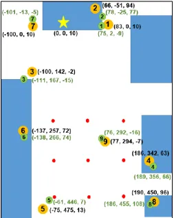
The best-case scenario for the calibration algorithm is examined using manually measured, or ground truth, locations of the offset detector and the 27 source locations. These locations were carefully measured by hand using measuring tapes and laser distance finder. The algorithm predicted offset detector location was compared to the ground truth measured offset detector location. The spherical shell thickness was chosen to be 4 cm, which produces results with the lowest Euclidean distance values for all count rate types and the most experiments. Figure 6 shows the results of recovering the algorithm predicted offset detector location compared to the ground truth measured offset detector location on an aerial schematic of the room where the measurements took place.
Fig. 6. Top-down view of the room in the x and y directions. The yellow star represents the known location of the co-located detector. Red dots represent the 27 source locations. Orange circles represent the ground truth measured offset detector locations and the green circles represent the calibration predicted offset detector locations. Blue blocks represent fixed lab furniture that may cause radiation scattering. Not to scale.
Table I shows these results. The Euclidean distance is of the predicted offset detector location to the ground truth offset detector location. The average Euclidean distance over the nine experiments using both gamma-ray and neutron data is 22.5 cm. When using only gamma-ray count rate data, the average Euclidean distance is 27.8 cm; and when using neutron only count rate data, the average Euclidean distance was 23.9 cm.
TABLE I
GROUND TRUTH CALIBRATION ALGORITHM RESULTS IN EUCLIDEAN DISTANCES
Exp.
No. Euclidean Distance: Combined Data (cm)
Euclidean Distance:
Photon Data (cm)
Euclidean Distance: Neutron Data (cm)
1 31.2 34.9 7.9
2 37.4 55.4 48.1
3 31.3 34.0 31.1
4 15.5 14.9 22.0
5 26.6 35.2 13.2
6 10.9 14.4 14.5
7 29.5 35.5 34.5
8 9.3 12.8 29.3
9 11.1 13.3 14.2
Absolute agreement is not necessarily required for the system to operate accurately. These algorithm-predicted locations are referred to as “pseudo-locations”. If there are significant room dependencies that are not easily captured by our allowed quadratic deviation from ideal radiation transport, then this deviation can possibly be incorporated into the model as a “best approximation” for the location of the radiological sensor vs. the radiation source location and the count rate response that will later be tracked in the system. Thus, the pseudo-locations will be utilized along with the non-ideal quadratic deviation. The distance discrepancy is the uncertainty in identifying the radiation detector’s location with respect to the overall radiation response from all the source locations compared to an idealized distance dependence of the detectable radiation flux, not the uncertainty in locating the source locations.
2) LiDAR Data
The HDL-32E covers a 360-degree view allowing all nine experiments to be analyzed. The HDL-32E’s location within the room allowed a view of all source locations, offset detector locations and the co-located detector. The spherical shell thickness was chosen to be 8 cm, which produces results with the lowest Euclidean distance values for all count rate types and the most experiments. Figure 7 shows the results of recovering the algorithm predicted offset detector location compared to the HDL-32E determined offset detector location on an aerial schematic of the room where the measurements took place.
Fig.7. Top-down view of the room in the x and y directions. The yellow star represents the known location of the co-located detector. Orange circles represent the HDL-32E measured offset detector locations and the green circles represent the calibration predicted offset detector locations. Not to scale.
Table II shows these where the Euclidean distance is from the predicted offset detector location to the HDL-32E determined detector location. The average Euclidean distance over all nine experiments using combined gamma-ray and neutron data is 21.8 cm. When using only gamma-ray count rate data, the average Euclidean distance is 25.5 cm; and when using neutron only count rate data, the average Euclidean distance was 21.9 cm.
TABLE II
GROUND TRUTH CALIBRATION ALGORITHM RESULTS IN EUCLIDEAN DISTANCES
Exp.
No. Euclidean Distance: Combined Data (cm)
Euclidean Distance: Photon Data (cm)
Euclidean Distance: Neutron Data (cm)
1 35.7 43.7 19.6
2 29.3 35.3 37.8
3 23.2 29.5 31.8
4 15.6 14.9 16.6
5 27.0 29.9 12.1
6 25.0 25.0 20.6
7 29.9 38.2 33.5
8 7.7 9.4 18.0
9 2.5 3.7 7.7
The results with the HDL-32E are close to the results obtained using the ground truth data. The HDL-32E has a range of up to 100 m with a typical accuracy of ±2 cm.
B. Correlation
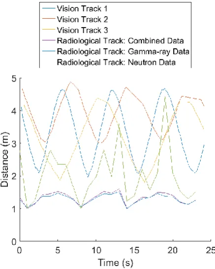
The count rate data for correlation was separated into one second time steps. Background was not removed from the data. Fig. 8shows vision and radiological tracks which are used for correlation.
Fig.8. Vision tracks of three persons to be correlated with the radiological track where the radiological track can be created from combined gamma-ray and neutron data, gamma-gamma-ray only data, or neutron only data.
Without subtracting background gamma-ray only data and combined data appear suppressed. This reduces the correlation between the radiological track and vision tracks. It is also important to note that the one over distance squared deviation shown in Fig. 3 can be used to adjust the radiological tracks. The following results, however, show the crude results of the two aforementioned correlation methods without background subtraction and without the use of the “pseudo-location”. In the future, results will be calculated with these additions and compared to the results presented here.
1) Cosine Distance Method
cps for both the co-located detector and the offset detector. These values vary slightly depending on room location. Background currently remains in the correlation data.
A. Calibration
The count rate used in the calibration, (1), is the net count rate with background subtracted. Measurement times are long enough such that the total rate error as a percentage is kept to around 2% for combined gamma-ray and neutron data.
1) Ground Truth Data
The best-case scenario for the calibration algorithm is examined using manually measured, or ground truth, locations of the offset detector and the 27 source locations. These locations were carefully measured by hand using measuring tapes and laser distance finder. The algorithm predicted offset detector location was compared to the ground truth measured offset detector location. The spherical shell thickness was chosen to be 4 cm, which produces results with the lowest Euclidean distance values for all count rate types and the most experiments. Figure 6 shows the results of recovering the algorithm predicted offset detector location compared to the ground truth measured offset detector location on an aerial schematic of the room where the measurements took place.
Fig. 6. Top-down view of the room in the x and y directions. The yellow star represents the known location of the co-located detector. Red dots represent the 27 source locations. Orange circles represent the ground truth measured offset detector locations and the green circles represent the calibration predicted offset detector locations. Blue blocks represent fixed lab furniture that may cause radiation scattering. Not to scale.
Table I shows these results. The Euclidean distance is of the predicted offset detector location to the ground truth offset detector location. The average Euclidean distance over the nine experiments using both gamma-ray and neutron data is 22.5 cm. When using only gamma-ray count rate data, the average Euclidean distance is 27.8 cm; and when using neutron only count rate data, the average Euclidean distance was 23.9 cm.
TABLE I
GROUND TRUTH CALIBRATION ALGORITHM RESULTS IN EUCLIDEAN DISTANCES
Exp.
No. Euclidean Distance: Combined Data (cm)
Euclidean Distance:
Photon Data (cm)
Euclidean Distance: Neutron Data (cm)
1 31.2 34.9 7.9
2 37.4 55.4 48.1
3 31.3 34.0 31.1
4 15.5 14.9 22.0
5 26.6 35.2 13.2
6 10.9 14.4 14.5
7 29.5 35.5 34.5
8 9.3 12.8 29.3
9 11.1 13.3 14.2
Absolute agreement is not necessarily required for the system to operate accurately. These algorithm-predicted locations are referred to as “pseudo-locations”. If there are significant room dependencies that are not easily captured by our allowed quadratic deviation from ideal radiation transport, then this deviation can possibly be incorporated into the model as a “best approximation” for the location of the radiological sensor vs. the radiation source location and the count rate response that will later be tracked in the system. Thus, the pseudo-locations will be utilized along with the non-ideal quadratic deviation. The distance discrepancy is the uncertainty in identifying the radiation detector’s location with respect to the overall radiation response from all the source locations compared to an idealized distance dependence of the detectable radiation flux, not the uncertainty in locating the source locations.
2) LiDAR Data
The HDL-32E covers a 360-degree view allowing all nine experiments to be analyzed. The HDL-32E’s location within the room allowed a view of all source locations, offset detector locations and the co-located detector. The spherical shell thickness was chosen to be 8 cm, which produces results with the lowest Euclidean distance values for all count rate types and the most experiments. Figure 7 shows the results of recovering the algorithm predicted offset detector location compared to the HDL-32E determined offset detector location on an aerial schematic of the room where the measurements took place.
Fig.7. Top-down view of the room in the x and y directions. The yellow star represents the known location of the co-located detector. Orange circles represent the HDL-32E measured offset detector locations and the green circles represent the calibration predicted offset detector locations. Not to scale.
Table II shows these where the Euclidean distance is from the predicted offset detector location to the HDL-32E determined detector location. The average Euclidean distance over all nine experiments using combined gamma-ray and neutron data is 21.8 cm. When using only gamma-ray count rate data, the average Euclidean distance is 25.5 cm; and when using neutron only count rate data, the average Euclidean distance was 21.9 cm.
TABLE II
GROUND TRUTH CALIBRATION ALGORITHM RESULTS IN EUCLIDEAN DISTANCES
Exp.
No. Euclidean Distance: Combined Data (cm)
Euclidean Distance: Photon Data (cm)
Euclidean Distance: Neutron Data (cm)
1 35.7 43.7 19.6
2 29.3 35.3 37.8
3 23.2 29.5 31.8
4 15.6 14.9 16.6
5 27.0 29.9 12.1
6 25.0 25.0 20.6
7 29.9 38.2 33.5
8 7.7 9.4 18.0
9 2.5 3.7 7.7
The results with the HDL-32E are close to the results obtained using the ground truth data. The HDL-32E has a range of up to 100 m with a typical accuracy of ±2 cm.
B. Correlation
The count rate data for correlation was separated into one second time steps. Background was not removed from the data. Fig. 8 shows vision and radiological tracks which are used for correlation.
Fig.8. Vision tracks of three persons to be correlated with the radiological track where the radiological track can be created from combined gamma-ray and neutron data, gamma-gamma-ray only data, or neutron only data.
Without subtracting background gamma-ray only data and combined data appear suppressed. This reduces the correlation between the radiological track and vision tracks. It is also important to note that the one over distance squared deviation shown in Fig. 3 can be used to adjust the radiological tracks. The following results, however, show the crude results of the two aforementioned correlation methods without background subtraction and without the use of the “pseudo-location”. In the future, results will be calculated with these additions and compared to the results presented here.
1) Cosine Distance Method
TABLE III
RESULTS OF THE COSINE DISTANCE METHOD Exp.
No. Ground Truth Trajectory
Correlation Between Radiation Data
and Ground Truth Trajectory
Selected
Trajectory Correlation Between Radiation Data and
selected Trajectory
1 1 0.9909 3 0.9942
2 3 0.9909 1 0.9964
3 2 0.9919 2 0.9919
4 1 0.9874 2 0.9939
5 3 0.9940 3 0.9940
6 2 0.9958 2 0.9958
7 2 0.9960 2 0.9960
8 3 0.9930 3 0.9930
9 3 0.9953 3 0.9953
10 2 0.9931 2 0.9931
11 2 0.9987 2 0.9987
2) Correlation Coefficient Method
Out of the 11 experiments, the correlation coefficient method chose the correct Trajectory seven times. Table IV shows the results. The “Ground Truth Trajectory” represents the trajectory of the person carrying the radioactive material and therefore is the trajectory that should be most correlated with the radiological data. The “Selected Trajectory” is the trajectory that the algorithm actually chose to be most correlated with the radiological data. The experiments where the algorithm chose the wrong trajectory are highlighted in red.
TABLE IV
RESULTS OF THE CORRELATION COEFFICIENT METHOD Exp.
No. Ground Truth Trajectory
Correlation Between Radiation Data
and Ground Truth Trajectory
Selected
Trajectory Correlation Between Radiation
Data and selected Trajectory
1 1 0.6150 2 0.7186
2 3 0.7240 3 0.7240
3 2 0.6195 2 0.6195
4 1 0.8543 1 0.8543
5 3 0.4152 3 0.4152
6 2 0.1064 1 0.3002
7 2 0.1622 1 0.2070
8 3 0.3718 3 0.3718
9 3 0.2686 3 0.2686
10 2 0.2857 2 0.2857
11 2 0.0948 1 0.8300
IV. CONCLUSION
Overall, the calibration algorithm for the vision/radiological system predicted the offset detector location well using ground truth and HDL-32E data. The uncertainty seen is within reason for tracking objects of size similar to people, luggage and packages. This calibration algorithm with be a good foundation when transitioning to a larger number of sensors or continuous (real-time) source movement used for calibrating the data fused system. Results of the two correlation methods were less ideal. The cosine distance only slightly more accurate than the correlation coefficient method. Each method proved to have difficulty predicting different experiment numbers only both predicted experiment one incorrectly. Subtracting background is likely to predict the correct track with better accuracy. Using
the calibration algorithm determined pseudo location may also improve the correlation algorithms ability to choose the correct track. The use of gamma-ray only data and neutron only data will also be examined. Other more complex and robust correlation algorithms are being looked into as well.
Transitioning to a real-time data processing system is in progress with anticipated challenges such as processing needs for 3D data. A high tracking and source identification accuracy have been achieved in initial stages approaching 90% accuracy in the early test scenarios. Another tracking scenario under investigation involves visual occlusions. In these experiments, a large structure is set in place to obstruct the view of the 3D vision sensor. Distance is then to be determined by the count rate data adjusting for the reduced count rate due to the obstruction. Multi-source tracking is an additional scenario where measurements have been taken are being analyzed. Dynamic scenes with a stationary source as well as scenes without a source entirely are also being explored. These measurements will assist in understanding and optimizing the system threshold. Many tracking scenarios are being studied to continue adjusting and improving the vision-aided detection system.
REFERENCES AND FOOTNOTES
[1] B.D. Geelhood, J.H. Ely, R.R. Hansen, R.T. Kouzes, J.E. Schweppe, and R.A. Warner, “Overview of Portal Monitoring at Border Crossings,” IEEE Conference Record, 2003.
[2] R. C. Runkle, T. M. Mercier, K. K. Anderson, and D. K. Carlson, "Point Source Detection and Characterization for Vehicle Radiation Portal Monitors,” IEEE Tans. Nucl. Sci., vol. 52, no. 6, pp. 3020-3025, 2005.
[3] S Brennan, A Mielke and D Torney, “Radiation detection with distributed sensor networks,” IEEE Computer Magazine, vol. 37, no. 8, pp. 57–59, 2004. [4] "Kinect for Windows Sensor Components and Specifications," Microsoft Developer Network. Microsoft, 2016. Web. 16 May 2016.
[5] Kadambi, Achuta, Vage Taamazyan, Boxin Shi, and Ramesh Raskar, "Polarized 3D: High-Quality Depth Sensing with Polarization Cues,"2015 IEEE International Conference on Computer Vision (ICCV) (2015): n. pag. MIT, Dec. 2015. Web. 17 May 2016.
[6]R. E. Kalman. A new approach to linear filtering and prediction problems. Journal of basic Engineering, 82(1):35–
45, 1960.