Mask-Constrained Power Synthesis of Large and Arbitrary Arraysas a Few-Samples Global Optimization

Mask-Constrained Power Synthesis of Large and Arbitrary Arrays

as a Few-Samples Global Optimization

Giada M. Battaglia1, Andrea F. Morabito1, Gino Sorbello2, and Tommaso Isernia1, *

Abstract—With reference to the mask-constrained power synthesis of shaped beams through

fixed-geometry antenna arrays, we elaborate a recently proposed approach and introduce an innovative effective technique. In particular, the proposed formulation, which can take into account mutual coupling and mounting platform effects, relies on a nested optimization where the external global optimization acts on the field’s phase shifts over a minimal number of ‘control points’ located into the target region whereas the internal optimization acts instead on excitations. As the internal optimization of the ripple is shown to result in a Convex Programming problem and the external optimization deals with a reduced number of unknowns, a full control of the shaped beam’s ripple and sidelobe level is achieved even in the case of arrays having a large size and aimed at generating large-footprint patterns. Examples involving comparisons with benchmark approaches as well as full-wave simulated realistic antennas are provided.

1. INTRODUCTION

The optimal synthesis of array antennas plays a key role in many fields of applied electromagnetics including satellite [1], radar [2], and cellular [3] telecommunications, as well as medical [4], electrical-energy [5] applications, and many further scenarios [6–22]. Amongst the different possible approaches to the problem, the ones guaranteeing the best exploitation of the available degrees of freedom (and hence the most effective use of the antenna resources) are those aiming at a ‘mask-constrained’ power synthesis. The latter consists in looking for square-amplitude distributions of the field lying between two arbitrary upper-bound and lower-bound functions [6].

In the case of fixed-geometry arrays (wherein the antenna layout is a-priori assigned while the elements’ excitations are the only unknowns), the problem has been solved in a globally-optimal fashion in both cases of pencil [7] anddifference [8] beams. In fact, without making any restriction on either the nature of the field or the excitations distribution or the array’s layout and shape, the synthesis has been cast as a Convex Programming (CP) or a Linear Programming (LP) problem. By so doing, it has been also possible to successfully address the ‘optimal compromise’ [9] among sum and difference patterns as well as the generation of phase-only reconfigurable sum and difference fields for monopulse radar telecommunications [10].

Unfortunately, quite different circumstances hold true for the synthesis ofshaped [11] beams, which still represents an unsolved canonical problem. In fact, leaving aside the approaches which do not exploit all the available degrees of freedom (such as the ones looking for pure-real fields [12] or unable to get a full control of the sidelobes [13]), the problem has been solved in a globally-optimal fashion only in the case where the sought power pattern is (or can be reduced to) a 1-D trigonometric polynomial. Currently,

Received 29 August 2019, Accepted 14 December 2019, Scheduled 23 December 2019

* Corresponding author: Tommaso Isernia ([email protected]).

this is indeed possible just for equispaced linear arrays [14], 1-D continuous sources [15],u-v factorable planar arrays [16], and circularly-symmetric sources and fields [17, 18]. Notably, these capabilities have also allowed developing interesting solutions for many other cases including, for instance, the isophoric arrays (see [22] for details concerning this particular architecture). In all the (very many) remaining instances, e.g., conformal arrangements of elements as well as arrays generating element-dependent radiation patterns (due to heterogeneity issues or to mutual-coupling and mounting-platform effects), only sub-optimal solutions seem to be available. In fact, the problem is usually tackled by resorting to a Global Optimization (GLO) of either the excitations or all the field samples (see for instance [19–21]). Hence, since in most cases the computational complexity of GLO procedures is expected to exponentially grow with the number of unknowns [23], it can prevent (in case of arrays composed by a large number of elements) the actual attainment of the global optimum.

A very recent approach partially overcoming the above difficulties is the one in [24]. In the latter, the main idea is to reduce the mask-constrained power synthesis of shaped beams to a number of CP problems by a-priori choosing the field’s phase shifts over a (minimal) [25, 26] number of ‘control points’ which are properly located over the shaped-beam region. The technique led to good results in benchmark cases (including the synthesis of generic arrays with whatever kind of geometry and completely-arbitrary element patterns) and showed interesting features such as the capability to determine (if any) a multiplicity of solutions all corresponding to the desired radiation power pattern. However, since the field’s phase shifts are explored in an enumerative fashion, the computational burden of that approach grows very rapidly with the number of control points, so that the computational burden is expected to be unpractical and/or not effective in case of large-footprint power patterns and large arrays. Moreover, the sampling of the phase shifts’ space which is needed for enumeration could be inadequate, thus possibly missing the global optimum.

In order to overcome the above problems, we further elaborate here on our previous approach [24]. In particular, we develop a nested optimization procedure where the external global optimization acts on the field’s phase shifts over a minimal number of ‘control points’ located into the target region whereas the internal optimization acts instead on excitations. Then, we show that as long as a given class of performance parameters (including ripple) is in order, the internal optimization reduces to a CP problem. Such a circumstance, along with the relatively small number of unknowns involved in the external optimization, allow a full control of the shaped beam’s ripple and sidelobe level in a number of cases (involving arrays having a large size and aimed at generating relatively large-footprint patterns) which cannot be solved in a globally-optimal fashion by the state-of-the-art techniques. In a nutshell, the proposed method identifies the phases of a few field samples as the actual reason for the non-convexity (and hence the difficulty) of the problem, and then elaborates on such a circumstance in order to deal with a global optimization problem having a number of unknowns as small as possible. Comparisons with [24] and many other methods confirm the interest and the effectiveness of the technique.

In the following, the approach is described in Section 2 while numerical examples involving large planar arrays and comparisons with several published techniques are shown in Section 3. Conclusions follow.

2. THE PROPOSED HYBRID APPROACH

In order to introduce the proposed approach, let us consider a region of interest Ω where r is the spatial variable, and an arbitrary array antenna composed of N generic elements. Also, let Ψ_n(r) be the Active Element Pattern (AEP) [27] of the n-th element, which takes into account the possible heterogeneity amongst the radiating elements as well as mutual coupling and mounting platform effects. As a consequence, the far-field distribution of the overall array can be written as:

F(r) = N

n=1

InΨn(r) (1)

ideas, let us suppose we are interested in minimizing the shaped-beam ripple in the region Λ. To this end, we set the approach’s basic bricks as follows:

i. given the array layout and AEPs, let us sample Λ intoL‘control points’rΛi, ...,rΛLat the Nyquist

distance [26]†;

ii. let us indicate with ϕi ∈ [−π,+π], i = 1, ..., L, the field phase shift between rΛi and rΛ1, and fix

to 0 the phase value attained by of the field in the point rΛ1 (which acts in the procedure as a

‘reference’ point)‡;

iii. note that the square of the power pattern’s ripple inside the shaped-beam region Λ can be expressed as:

R(I1, ..., In, ϕ1, ..., ϕL) =

P(r)−P(r)2 (2)

where P(r) = |F(r)|2 and P(r) = [U B(r) +LB(r)]/2. Therefore, for any fixed L-tuple ϕ1, ..., ϕL, R

is a fourth-order polynomial of the unknownsI1, ..., In. This notwithstanding, we show in Appendix A

that, by a proper choice of the sampling points (and sampling representations), such a function can be considered to be substantially convex with respect to the field samples (and hence to the excitations, which linearly depends on them).

On the basis of all the above and by denoting as|F|desired_i the desired value for the field amplitude at thei-th control point, the overall problem can be conveniently set as:

min ϕ1, ..., ϕL

min I1, ..., In

r∈Λ

R(r)dr (3)

where the internal problem is subject to the following constraints:

R{F(rΛi)} =|F|desired_i cosϕi i= 1, ..., L (4) I{F(rΛi)} =|F|desired_i sinϕi i= 1, ..., L (5)

|F(r)|2 ≤U B(r) ∀r∈Ω\Λ (6)

P +√R ≤U B(r) ∀r∈Λ (7)

where, by virtue of the definition ofP, the constraint (7) also entails that |F(r)|2 ≥LB(r). A number of comments are now in order.

Let us first note that, for any fixed value ofϕ1, ..., ϕL, constraints (4)–(5) are equivalent to enforce

|F(rΛi)|=|F|desired_i ∀i, and hence a proper choice of|F|desired1 , ...,|F|desiredL , and the use of constraints [7],

allows shaping the power pattern inside the region of interest. Also note that one can eventually use bounds (rather than fixed quantities) for|F|desired1 , ...,|F|desiredL . At the same time, constraints (6) allow

keeping under control the sidelobes’ behavior outside Λ. Hence, in summary:

• inside the target region Λ, constraints (4) and (5) are used to ensure that the field amplitude attains a precise value on each of the control points while constraint (7) allows ensuring that its ripple does not exceed a given threshold;

• outside the target region Λ, constraint (6) allows keeping under control the sidelobes’ behavior. Notably, constraints (4)–(5) and (6) respectively are linear forms and a positive semi-definite quadratic form of the excitations. Then, provided R can be considered to be quadratic (which can be eventually enforced by a denser sampling — see Appendix A), constraints (7) and the objective function (3) are also convex, so that the overall problem is a CP one, with the inherent advantages in terms of solutions’ optimality and computational burden. In particular, for any fixed value ofϕ1, ..., ϕL

and |F|desired1 , ...,|F|desiredL , it admits a single minimum (if any), which is therefore the global optimum.

In Eq. (3) the external minimization will require a GLO tool on a reduced number of unknowns, whereas the internal minimization can be solved by means of a fast local-optimization. In summary, the synthesis is conveniently decomposed into two nested parts, i.e., a GLO on L variables and a CP optimization of the N excitations. It is also worth noting that the cost function (3) can be eventually † _{While this criterion will allow avoiding any redundancy, other choices (such as involving the so-called ‘self-truncating’ sampling}

series [28] — see also Appendix A) are possible.

substituted by other convex cost functions such as for instance the maximum value ofR(r) [i.e., using a

minimax criterion on the ripple rather than the one in (3)] or the overall radiated power (which would optimize directivity) without affecting the CP nature of the overall problem.

The proposed approach exploits the partial convexity§of the overall synthesis problem with respect to the excitations in order to reduce the dimensionality of the global optimization problem. In fact, the GLO algorithm must deal only with the few (auxiliary) variables in which the overall problem is not convex, i.e., the phase shifts, with a decisive, beneficial effect on both the computational time and the reliability of the obtained results. In fact, the exploitation of a GLO on just the ‘non-convex part’ of the problem will allow avoiding sub-optimal solutions, i.e., local minima of the objective function. Moreover, since the required value of L is generally much lower than N, the computational burden of the proposed synthesis procedure will be lower than the one of any GLO algorithm acting on either

all of the field samples or the array excitations. Finally, possible discretization errors arising in the enumerative technique [24] are also avoided. As a consequence of all the above, the proposed strategy is much more effective than the one recently introduced in [24] which, however, was able to identify a multiplicity of solutions.

In the following Section, we prove the validity of the approach in a number of (benchmark) test cases of actual interest where the enumerative search exploited in [24] is not adequate (Subsection 3.1) as well as in the not-trivial case where AEPs (rather than identical isolated element patterns) have to be considered (Subsection 3.2).

3. NUMERICAL EXAMPLES

In this Section, we report some numerical examples concerning the synthesis of large planar arrays. In particular, in Subsection 3.1 we provide comparisons with the procedures respectively published in [14, 29, 30], while in Subsection 3.2 we consider a realistic array of truncated waveguides with full-wave simulated AEPs.

In order to deal with a number of unknown phase shifts as small as possible, we basically consider a Nyquist sampling for the choice of the control points. Small displacements have been anyway used in some cases (as indicated) in order to get a better matching with the mask requirements.

The internal and external parts of the minimization (3) have been respectively performed thorough the fmincon and ga routines of MATLAB (version R 2016B). Also note that an optimal choice of the external global optimization procedure is outside of the scope of the proposed general approach.

In all experiments, the radiating system has been set as an equispaced planar array composed by a different number of elements along the xand y axes, and the rcoordinate has been expressed through the usual spectral variables u and v, i.e., u = βdxsinθcos Φ and v = βdysinθsin Φ [where β = 2π/λ denotes the wavenumber (λ being the operative wavelength), (dx, dy) are the element spacings along thexandy axis, and (θ, Φ) respectively denote the elevation and azimuth aperture angles with respect to boresight). Moreover, we set |F|desired_i = 1∀i.

The radiation performances have been evaluated by means of the ‘peak-to-trough’ ripple (PTR) (defined as the ratio between the maximum and the minimum value attained by the power pattern ∀r∈Λ), the ‘peak’ sidelobe level (PSL) (defined as the ratio between the maximum value attained by the power pattern ∀r ∈ Ω\Λ and the power pattern’s absolute maximum), and the Dynamic Range Ratio (DRR) (defined as the ratio amongst the maximum and minimum amplitudes of the excitations). In particular, for each example, we report the achieved values for these parameters in two different cases, i.e.:

• case (a), when using the basic formulation of the synthesis problem;

• case (b), when adding to the stopping rule of ga an upper-bound constraint on DRR and turning off (i.e., erasing) the antennas having a very-small excitation amplitude.

3.1. Comparison with Some Existing Approaches

In the first example, we considered the same array and power mask as the ones adopted in [14, 24], i.e.:

• a square equispaced array withN = 225 isotropic elements located along the xand y axes with a 0.5λ spacing;

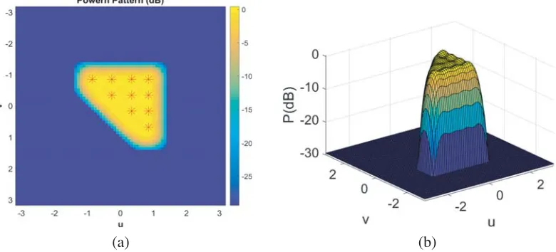
• the power mask shown in Fig. 10 of [14], which enforces a triangular footprint with PTR = 1 dB. In order to get the desired shaping, L = 10 control points have been located inside the region Λ as described by Fig. 1(a). The square amplitude of the complex field synthesized through the proposed approach is shown in Fig. 1, while Table B1 reports the complex excitations set corresponding to it. The presented method provided {DRR = 144, PTR = 1 dB, PSL = −29.4 dB} in the case (a), and {DRR = 97, PTR = 1 dB, PSL =−29 dB}in the case (b) by erasing the 7 elements having the lowest

(a) (b)

Figure 1. Synthesis of a 225-elements array generating a flat-top beam with a triangular footprint

(comparison with [14]) when using the excitations reported in Table B1: (a) 2-D and (b) 3-D power-patterns representations. Control points’ locations [marked in red in subplot (a)]: (u, v) = {(−0.85,−0.85),(−0.25,−0.85),(0.35,−0.85),(0.85,−0.85),(−0.25,−0.34),(0.34,−0.34),(0.85,−0.34),

(0.34,0.17),(0.85,0.17),(0.85,0.68)}.

(a) (b) (c)

Figure 2. Synthesis of a 156-elements array generating a flat-top power pattern having a square

footprint (comparison with [29]) when using the excitations reported in Table B2: (a) array layout, where only the elements internal to the circle of radius 3.5λ(i.e., depicted in red color) are used; (b) 2-D and (c) 3-D views of the power pattern. Control points’ locations [marked in red in subplot (b)]: (u, v) = {(0.26,−0.26),(0.78,−0.26),(−0.26,−0.26),(−0.78,−0.26),(0.26,−0.78),(0.78, −0.78),(−0.26, −0.78),

(−0.78,−0.78), (−0.78,0.26), (−0.26,0.26), (0.26,0.26), (0.78,0.26), (−0.78,0.78), (−0.26,0.78),

excitation amplitude. Therefore, in the latter case, as compared to the results in [14] (i.e., DRR = 20, PTR = 1 dB, PSL =−28 dB) the approach provided a lower PSL and a larger DRR. Moreover, since it allows the straightforward determination of the array excitations, the present approach is both much easier to implement and much faster than the one in [14]. Finally, the computational burden was considerably reduced with respect to [24], where in fact we needed to enforce some symmetry on the complex pattern in order to halve the number of control points (with a consequent loss of degrees of freedom).

In the second test case, we compared the proposed technique to the one in [29] by pursuing similar power-pattern goals through an array composed of a lower number of elements. In particular, starting from a 16×16 grid (withdx =dy = 0.5λ), an array composed ofN = 208 elements has been considered in [29] by erasing all the antennas external to the circle of radius 4λ. Conversely, by starting from the same uniform grid but using a circle of radius 3.5λ (see Fig. 2) in order to discard some elements, we achieved a layout composed of 156 elements. All the element patterns have been set as isotropic and, in the same way as in [29], the mask has been designed in such a way to generate a flat-top beam with a square footprint covering the region (|u|<0.25, |v|<0.25) and guaranteeing a PSL =−20.6 dB for (|u|>0.3125, |v|>0.3125).

The L = 16 adopted control points are depicted in Fig. 2(b), while the excitations identified through the proposed approach are reported in Table B2 and the corresponding power pattern is shown

(a) (b) (c)

(d) (e) (f)

Figure 3. Synthesis of a 400-elements array devoted to covering the mainland of China

(com-parison with [30]): (a), (b) map and mask (courtesy of the authors of [30]); (c) 2-D plot of the achieved power pattern and the exploited control points; (d) amplitude and (e) phase of the synthesized excitations; (f) 3-D power pattern view. Control points’ locations [marked in red in subplot (c)]: (u, v) = {(−0.06,0.66),(0.25,0.66),(0.56,0.66),(−0.38,0.34),(−0.06,0.34),(0.25,0.34),(0.56,0.34),(−0.69,0.03),

(−0.38,0.03),(−0.06,0.03),(0.25,0.03),(0.56,0.03),(−0.69,−0.28),(−0.38,−0.28),(−0.06,−0.28),(0.25,

in Fig. 2(b) (2-D plot) and in Fig. 2(c) (3-D plot). The presented method provided{DRR = 174, PTR = 0.3 dB, PSL =−20.6 dB} in the case (a), and {DRR = 19, PTR = 0.45 dB, PSL =−20.6 dB} in the case (b) by erasing the 6 elements having the lowest excitation amplitude. Therefore, in the latter case, as compared to the best results in [29] (i.e., DRR = 24.4, PTR = 0.3 dB, PSL =−20.6 dB), the proposed approach allowed to save the 22.5% of elements while guaranteeing the same PSL and beam footprint, a slightly lower DRR, and a slightly larger PTR. As in the previous test case, the adopted mask and the synthesis goals resulted unaffordable by the approach in [24] (where it was possible to exploit only a quarter of the control points adopted herein).

As the third test case, we provide a comparison with the method recently published in [30]. In particular, we considered the same array and specifications as the ones adopted therein, i.e., aN = 400 elements square array (composed by 20×20 isotropic antennas located on the x and y axes with a constant 0.5λ spacing) as well as a mask pursuing a uniform coverage of the mainland of China (see Fig. 3, and also Fig. 7 of [30]).

To get the desired shaping,L= 19 control points have been uniformly set within the target area as reported in Fig. 3(c). The 2-D and 3-D plots of the achieved power-pattern distribution are respectively shown in Fig. 3(c) and Fig. 3(f). The amplitude and phase of the corresponding excitations (whose table is not reported for length and readability issues) are depicted in Fig. 3(d) and Fig. 3(e), respectively.

(a) (b)

(c) _(d)

Figure 4. Full-wave synthesis of a realistic array generating a flat-top beam having an elliptical

The presented method provided {DRR = 10000, PTR = 0.12 dB, PSL = −27.9 dB} in the case (a), and {DRR = 198, PTR = 1 dB, PSL =−27.9 dB} in the case (b). Therefore, in the latter case, it favorably compares to one in [30] by allowing equal PSL performances, a PTR reduction from 1.4 to 1.0 dB and, at the same time, a DRR decrease from 1000 to 198. Finally, it is worth noting that the number of control points required to realize the China coverage definitively excludes the enumerative technique developed in [24].

3.2. Full-Wave Synthesis of a Realistic Array

As a final numerical experiment, we tested the proposed technique for the full-wave synthesis of a

N = 100 elements planar array equal to the one considered (for different purposes) in [31, 32], i.e., composed by 10×10 truncated waveguides uniformly spaced withdx=λand dy = 0.5λ. In particular, WR90 waveguides having a size of 22.86 ×10.16 mm2, operating at 10 GHz, truncated without any flaring, and mounted on an infinite ground plane were used [see Fig. 4(c)].

First, in order to perform the synthesis, the AEPs have been computed by CST Microwave Studio full-wave simulations. Some of them, whose heterogeneity prevents one from using any technique relying on the array factor concept or trigonometric polynomials,are reported in Fig. 4(d). Then, the ripple has been minimized within the ellipsoidal shaped target area of axes (sinθcos Φ,sinθsin Φ) = (0.22,0.42) while pursuing a PSL =−20 dB outside the ellipsoidal area of axes (sinθcos Φ,sinθsin Φ) = (0.45,0.86). To this end,L= 5 control points have been uniformly set within the target area as reported in Fig. 4(a). Figures 4(a) and 4(b) respectively show the 2-D and 3-D plots of the synthesized power pattern, while Table B3 reports the excitations corresponding to it. The PTR and DRR turned out being equal to 0.28 dB and 32.2, respectively.

4. CONCLUSIONS

An approach aimed at synthesizing shaped patterns subject to arbitrary sidelobe bounds by means of generic fixed-geometry arrays has been presented and tested on several benchmark cases. The proposed technique is based on the exploitation of some hidden convexity property, auxiliary variables, and nested optimization.

As discussed and validated through examples, the approach is very effective even in those cases where the previous methods based on either enumerative strategies or global optimizations on all the excitations (or field samples) result too heavy under the computational point of view. In fact, the global optimization is here performed on a minimal number of unknowns (which are conveniently identified as the field phase in a low number of control points). By so doing, the computational burden required for optimizing the synthesis is reduced as much as possible.

The new approach is also very general and overcomes the limitations of the Woodward-Lawson-related techniques (which do not exploit the degrees of freedom arising from the field’s phase shifts) as well as of all methods requiring that the field is expressible as a 1-D trigonometric polynomial.

APPENDIX A.

This Appendix is aimed at showing how the R function (2) [and correspondingly the cost function (3)] can be accurately approximated as a positive semi-definite quadratic function of the excitations. To this end, as a linear transformation does not affect convexity properties, let us consider a sampling representation of the field. By so doing, one can rewrite expression (1) as follow:

|F(r)|2 =

L

m=1

FmS(r−r_m) + Q

k=1

FkS(r−r_k)

2

(A1)

whereinQis the number of Nyquist samples located in Ω\Λ;S(r−r_m) are the chosen sampling functions; and Fi denotes the value of the field in the sampling pointri. Notably, the first addend [say FDOM(r)]

is known (as field samples have been fixed) while the second addend [say FRES(r)] is the one actually

sampling functions as well as of the fact that it depends on the (low-amplitude) sidelobes’ samples, the second term can be considered to be negligible (residual) with respect to the first one. Then, by further elaborating Eq. (A1), one finds:

|F(r)|2 = |FDOM(r)|2+ 2R{FDOM(r)FRES∗ (r)}+|FRES(r)|2 (A2)

wherein the first (and dominant) term is constant, the second term is a linear function of the unknowns, and the third one is a quadratic form of the unknowns. Hence, as long as the quadratic part can be neglected with respect to the previous ones, one can conclude that Eq. (2) is well approximated (within a controlled accuracy) by a positive semidefinite quadratic form, and hence by a convex function. Also note that the third and last term can be made smaller and smaller (paying a price in terms of number of samples) by a proper use of the self-truncating sampling functions discussed in [28].

APPENDIX B.

The aim of this Appendix is to report the excitation values determined by using the proposed approach.

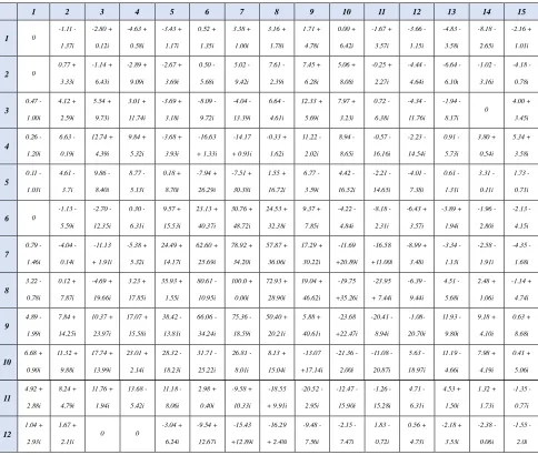
Table B1. Complex excitation coefficients for the design of a 225-elements array generating a flat-top

beam having a triangular contour as per Fig. 1 (first numerical example).

1 2 3 4 5 6 7 8 9 10 11 12 13 14 15

1 0

-1.11 - 1.37i -2.80 + 0.12i -4.63 + 0.58i -3.43 + 1.17i 0.52 + 1.35i 3.38 + 1.00i 3.16 + 1.78i 1.71 + 4.78i 0.00 + 6.42i -1.67 + 3.57i -3.66 - 1.15i -4.83 - 3.58i -8.18 - 2.65i -2.16 + 1.01i

2 0

0.77 + 3.33i -1.14 + 6.43i -2.89 + 9.09i -2.67 + 3.69i 0.50 - 5.68i 5.02 - 9.42i 7.61 - 2.39i 7.45 + 6.28i 5.06 + 8.08i -0.25 + 2.27i -4.44 - 4.64i -6.64 - 6.10i -1.02 - 3.16i -4.18 - 0.78i 3 0.47 - 1.00i 4.12 + 2.59i 5.54 + 9.73i 3.01 + 11.74i -3.69 + 3.18i -8.09 - 9.72i -4.04 - 13.39i 6.64 - 4.61i 12.33 + 5.69i 7.97 + 3.23i 0.72 - 6.38i -4.34 - 11.76i -1.94 - 8.17i 0 4.00 + 3.45i 4 0.26 - 1.20i 6.63 - 0.19i 12.74 + 4.39i 9.84 + 5.32i -3.68 + 3.93i -16.63 + 1.33i -14.17 + 0.91i -0.33 + 1.62i 11.22 - 2.02i 8.94 - 8.65i -0.57 - 16.16i -2.23 - 14.54i 0.91 - 5.73i 3.80 + 0.54i 5.34 + 3.58i 5 0.11 - 1.03i 4.61 - 3.7i 9.86 - 8.40i 8.77 - 5.13i 0.18 + 8.70i -7.94 + 26.29i -7.51 + 30.38i 1.55 + 16.72i 6.77 - 3.59i 4.42 - 16.52i -2.21 - 14.65i -4.01 - 7.38i 0.61 - 1.31i 3.31 - 0.11i 1.73 - 0.71i

6 0

13 -3.56 + 3.02i -2.46 + 2.23i -2.88 + 4.92i -6.09 + 8.76i -8.92 + 10.51i -9.90 + 7.17i -5.76 - 0.72i 1.17 - 3.98i 4.34 - 0.30i 3.18 + 6.29i -1.28 + 8.92i -3.61 + 5.06i -2.54 + 0.52i -0.52 - 0.89i 0 14 -4.82 + 2.17i -2.26 + 3.09i -1.63 + 7.28i -3.26 + 10.27i -7.29 + 6.46i -5.84 - 3.56i 1.77 - 10.21i 10.42 - 5.78i 10.88 + 6.24i 2.81 + 12.33i -4.78 + 7.65i -4.35 + 0.04i -0.29 - 2.47i 1.85 - 0.68i 0.09 + 2.17i 15 -4.33 - 1.42i -0.49 + 2.65i 1.80 + 4.86i 0.15 + 4.25i -3.62 + 0.14i -4.04 - 6.15i 2.19 - 7.78i 8.20 - 1.80i 7.23 + 5.56i 0.14 + 7.25i -4.24 + 2.40i -3.04 - 2.67i 1.41 - 3.45i 3.72 - 1.29i 0.98 + 2.17i

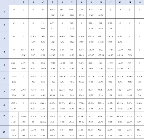
Table B2. Complex excitation coefficients for the design of a 156-elements array generating a flat-top

beam having a square contour as per Fig. 2 (second numerical example).

1 2 3 4 5 6 7 8 9 10 11 12 13 14

1 0 0 0 0 8.95 +

5.09i 3.65 – 2.96i 0.05 – 10.8i -2.13 – 12.93i -6.18 – 14.43i 4.26 – 10.46i

0 0 0 0

2 0 0 0 4 +

4.99i

4.47 –

0.5i

0 -4.06 +

2.17i

0 -4.86 +

1.19i

-5.99 –

5.45i

10.45 –

2.74i

0 0 0

3

0 0 -3.36 –

4.48i 2.48 – 8.86i -2.6 – 6.82i -4.64 – 4.11i -7.34 + 6.03i -8.98 + 9.53i -7.83 + 12.08i -13.13 + 6.39i -11.1 + 0.04i 0.5 – 5.98i 0 0 4

0 3.88 +

4.84i 2.46 – 8.87i -5.19 – 12.14i -10.26 –12.92i -11.17 – 0.78i -8.73 + 16.42i -9.14 + 31.61i -10.59 +29.67i -10.21 +22.38i -16.87 + 8.07i -13.17 – 6.31i -9.31 – 7.88i 0 5 8.86 + 5.05i 4.57 – 0.51i -2.6 – 6.82i -10.26 –12.92i -13.77 – 9.09i -12.04 + 1.2i -2.32 + 18.66i -0.03 + 32.5i -0.02 + 31.6i -2.98 + 23.61i -14.83 + 8.71i -11.89 + 0.56i -9.86 – 6.1i 0 6 3.57 – 2.91i

0 -4.65 –

4.1i -11.17 – 0.77i -12.04 + 1.2i -2.68 + 4.46i 12.62 + 7.54i 20.37 + 13.43i 20.17 + 11.46i 15.4 + 11.97i 2.14 + 9.26i -4.77 + 6.91i -6.13 + 4.99i 0.54 + 4.06i 7 0.05 – 10.9i -3.96 + 2.13i -7.34 + 6.03i -8.73 + 16.42i -2.3 + 18.56i 12.53 + 7.49i 31.36 – 5.85i 41.39 – 18.41i 45.53 – 16.72i 34.79 – 5.35i 19.38 + 9.53i 5.12 + 16.63i 2.02 + 13.45i -0.02 + 5.9i 8 -2.27 – 13.81i

0 -8.98 +

9.53i -9.14 + 31.61i -0.03 + 32.6i 20.37 + 13.43i 41.39 – 18.41i 57.89 – 41.45i 62.48 – 41.48i 50.75 – 19.32i 36.03 + 5.15i 13.92 + 23.71i 7.63 + 21.06i -0.66 + 5.66i

9 _{-6.1 – -4.66 + -7.78 + -10.56 -0.02 + 20.17 + 45.34 – 62.48 – 67 – 51.09 – 33.45 + 13.56 + 4.77 + 0.75 +}

14.25i 1.15i 12i +29.57i 31.6i 11.46i 16.65i 41.48i 39.35i 18.39i 9.22i 22.19i 21.37i 8.17i

11 0 10.25 – 2.69i -11.1 + 0.03i -16.87 + 8.07i -14.84 + 8.7i 2.14 + 9.26i 19.38 + 9.54i 36.03 + 5.14i 33.45 + 9.21i 17.25 + 8.43i 11.5 + 15i -3.07 + 11.6i -11.85 + 6.67i 0

12 0 0 0.5 –

5.98i -13.16 – 6.31i -11.99 + 0.56i -4.78 + 6.91i 5.12 + 16.63i 13.93 + 23.71i 13.55 + 22.19i 9.57 + 20.25i -3.07 + 11.6i -23.39 + 2.25i 0 0

13 0 0 0

-9.31 – 7.89i -9.95 – 6.16i -6.12 + 4.99i 2 + 13.35i 7.6 + 20.97i 4.76 + 21.38i 1.13 + 18.27i -11.85 + 6.67i

0 0 0

14

0 0 0 0 0 0.54 +

4.06i -0.01 + 6i -0.63 + 5.36i 0.76 + 8.17i 2.78 + 4.63i

0 0 0 0

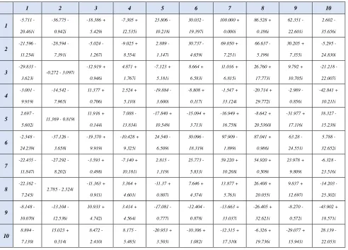
Table B3. Complex excitation coefficients achieved in the full-wave synthesis of a 100-elements realistic

array generating a uniform-amplitude field with an elliptical footprint as per Fig. 4 (fourth numerical example).

1 2 3 4 5 6 7 8 9 10

1 -5.711 - 20.461i -36.775 - 0.942i -18.386 + 5.429i -7.305 + 12.535i 23.806 - 10.218i 30.032 - 19.397i 100.000 + 0.000i 86.528 + 0.186i 62.351 - 22.601i 2.602 - 35.656i 2 -21.596 - 11.254i -28.594 - 7.391i -5.024 - 1.267i -9.025 + 8.554i 2.889 - 1.147i 30.737 - 4.659i 69.050 + 7.251i 66.637 - 5.199i 30.205 + 7.355i -5.295 - 24.830i 3 -29.833 - 3.623i

-0.272 - 3.097i

-12.919 + 0.946i 4.871 + 1.767i -7.123 + 5.181i 8.664 + 6.583i 11.016 + 6.815i 26.760 + 17.773i 9.792 + 10.705i -21.218 - 22.007i 4 -3.001 - 9.919i -14.542 - 7.965i 11.377 + 0.706i 2.524 + 5.110i -19.884 - 3.600i -8.808 + 0.117i -1.547 + 33.124i -20.714 + 29.772i -2.989 - 0.856i -42.841 + 10.211i 5 2.697 - 5.602i

11.369 - 0.819i

11.916 + 0.144i 7.088 - 13.834i -17.840 + 10.549i -15.094 + 3.713i -16.949 + 16.758i -8.642 + 20.5360i -31.977 + 17.116i 18.327 - 15.238i 6 -2.348 - 24.239i -37.126 - 3.658i -19.370 + 9.919i -10.428 + 9.325i 24.540 - 6.509i 30.096 - 18.319i 97.909 - 1.899i 87.041 + 0.986i 63.28 - 24.551i 5.788 - 32.652i 7 -22.455 - 11.847i -27.292 - 8.202i -3.593 + 0.498i -7.140 + 10.181i 2.815 - 1.319i 25.773 - 5.833i 59.220 + 10.268i 54.920 + 0.509i 23.978 + 9.809i -6.328 - 23.516i 8 -22.162 - 7.245i

2.785 - 2.324i

REFERENCES

1. Morabito, A. F., A. R. Lagan`a, and L. Di Donato, “Satellite multibeam coverage of earth: Innovative solutions and optimal synthesis of aperture fields,” Progress In Electromagnetics Research, Vol. 156, 135–144, 2016.

2. Mosalanejad, M., S. Brebels, C. Soens, I. Ocket, and G. A. E. Vandenbosch, “Millimeter wave cavity backed microstrip antenna array for 79 GHz radar applications,” Progress In Electromagnetics Research, Vol. 158, 89–98, 2017.

3. Dessouky, M. I., H. A. Sharshar, and Y. A. Albagory, “Design of high altitude platforms cellular communications,”Progress In Electromagnetics Research, Vol. 67, 251–261, 2007.

4. Iero, D. A. M., T. Isernia, A. F. Morabito, I. Catapano, and L. Crocco, “Optimal constrained field focusing for hyperthermia cancer therapy: A feasibility assessment on realistic phantoms,”Progress In Electromagnetics Research, Vol. 102, 125–141, 2010.

5. Morabito, A. F., “Synthesis of maximum-efficiency beam arrays via convex programming and compressive sensing,”IEEE Antennas and Wireless Propagation Letters, Vol. 16, 2404–2407, 2017. 6. Isernia, T. and A. F. Morabito, “Mask-constrained power synthesis of linear arrays with even excitations,” IEEE Transactions on Antennas and Propagation, Vol. 64, No. 7, 3212–3217, 2016. 7. Isernia, T. and G. Panariello, “Optimal focusing of scalar fields subject to arbitrary upper bounds,”

Electronics Letters, Vol. 34, No. 2, 162–164, 1998.

8. Bucci, O. M., M. D’Urso, and T. Isernia, “Optimal synthesis of difference patterns subject to arbitrary sidelobe bounds by using arbitrary array antennas,” IEE Proceedings on Microwaves, Antennas and Propagation, Vol. 152, No. 3, 129–137, 2005.

9. Oliveri, G. and L. Poli, “Optimal sub-arraying of compromise planar arrays through an innovative ACO-weighted procedure,” Progress In Electromagnetics Research, Vol. 109, 279–299, 2010. 10. Morabito, A. F. and P. Rocca, “Reducing the number of elements in phase-only reconfigurable

arrays generating sum and difference patterns,”IEEE Antennas and Wireless Propagation Letters, Vol. 14, 1338–1341, 2015.

11. Orchard, H. J., R. S. Elliott, and G. J. Stern, “Optimizing the synthesis of shaped beam antenna patterns,” IEE Proceedings H — Microwaves, Antennas and Propagation, Vol. 132, No. 1, 63–68, 1985.

12. Zhang, T. and W. Ser, “Robust beampattern synthesis for antenna arrays with mutual coupling effect,” IEEE Transactions on Antennas and Propagation, Vol. 59, No. 8, 2889–2895, 2011. 13. Woodward, P. and J. Lawson, “The theoretical precision with which an arbitrary radiation-pattern

may be obtained from a source of finite size,” Journal of the Institution of Electrical Engineers — Part III: Radio and Communication Engineering, Vol. 95, No. 37, 363–370, 1948.

14. Isernia, T., O. M. Bucci, and N. Fiorentino, “Shaped beam antenna synthesis problems: Feasibility criteria and new strategies,” Journal of Electromagnetic Waves and Applications, Vol. 12, No. 1, 103–137, 1998.

15. Morabito, A. F., T. Isernia, and L. Di Donato, “Optimal synthesis of phase-only reconfigurable linear sparse arrays having uniform-amplitude excitations,”Progress In Electromagnetics Research, Vol. 124, 405–423, 2012.

16. Morabito, A. F., A. Massa, P. Rocca, and T. Isernia, “An effective approach to the synthesis of phase-only reconfigurable linear arrays,”IEEE Transactions on Antennas and Propagation, Vol. 60, No. 8, 3622–3631, 2012.

17. Bucci, O. M., T. Isernia, and A. F. Morabito, “Optimal synthesis of circularly symmetric shaped beams,”IEEE Transactions on Antennas and Propagation, Vol. 62, No. 4, 1954–1964, 2014. 18. Morabito, A. F., T. Isernia, and A. R. Lagan`a, “On the optimal synthesis of ring symmetric shaped

patterns by means of uniformly spaced planar arrays,” Progress In Electromagnetics Research B, Vol. 20, 33–48, 2010.

20. Wang, W.-B., Q. Feng, and D. Liu, “Application of chaotic particle swarm optimization algorithm to pattern synthesis of antenna arrays,” Progress In Electromagnetics Research, Vol. 115, 173–189, 2011.

21. Liu, D., Q. Feng, W.-B. Wang, and X. Yu, “Synthesis of unequally spaced antenna arrays by using inheritance learning particle swarm optimization,”Progress In Electromagnetics Research, Vol. 118, 205–221, 2011.

22. Bucci, O. M., T. Isernia, A.F. Morabito, S. Perna, and D. Pinchera, “Aperiodic arrays for space applications: An effective strategy for the overall design,” Proceedings of the 3rd European Conference on Antennas and Propagation, EuCAP 2009, 2031–2035, Berlin, Germany, March 23– 27, 2009.

23. Floudas, C. A. and P. M. Pardalos,State of the Art in Global Optimization: Computational Methods and Applications, IX, Kluwer Acad. Publ., New York, Dordrecht, 1996.

24. Battaglia, G. M., G. G. Bellizzi, A. F. Morabito, G. Sorbello, and T. Isernia, “A general effective approach to the synthesis of shaped beams for arbitrary fixed-geometry arrays,” Journal of Electromagnetic Waves and Applications, Vol. 33, No. 18, 2404–2422, 2019.

25. Morabito, A. F., L. Di Donato, and T. Isernia, “Orbital angular momentum antennas: Understanding actual possibilities through the aperture antennas theory,” IEEE Antennas and Propagation Magazine, Vol. 60, No. 2, 59–67, 2018.

26. Bucci, O. M., C. Gennarelli, and C. Savarese, “Representation of electromagnetic fields over arbitrary surfaces by a finite and nonredundant number of samples,” IEEE Transactions on Antennas and Propagation, Vol. 46, No. 3, 351–359, 1998.

27. Morabito, A. F., A. Di Carlo, L. Di Donato, T. Isernia, and G. Sorbello, “Extending spectral factorization to array pattern synthesis including sparseness, mutual coupling, and mounting platform effects,” IEEE Transactions on Antennas and Propagation, Vol. 67, No. 7, 4548–4559, 2019.

28. Bucci, O. M. and G. Di Massa, “The truncation error in the application of sampling series to electromagnetic problems,”IEEE Transactions on Antennas and Propagation, Vol. 36, No. 7, 941– 949, July 1988.

29. Rodriguez, A., R. Munoz, H. Estevez, F. Ares, and E. Moreno, “Synthesis of planar arrays with arbitrary geometry generating arbitrary footprint patterns,”IEEE Transactions on Antennas and Propagation, Vol. 52, No. 9, 2484–2488, 2004.

30. Qi, Y. X. and J. Y. Li, “Superposition synthesis method for 2-D shaped-beam array antenna,”

IEEE Transactions on Antennas and Propagation, Vol. 66, No. 12, 6950–6957, 2018.

31. Fuchs, B., L. Le Coq, and M. D. Migliore, “Fast antenna array diagnosis from a small number of far-field measurements,”IEEE Transactions on Antennas and Propagation, Vol. 64, No. 6, 2227–2235, 2016.