Electromagnetic Scattering Analysis for Two-Dimensional Gaussian
Rough Surfaces with Texture Characteristics Using
Small-Slope Approximation Method
Rong-Qing Sun*, Jing Xie, and Yang-Wei Zhang
Abstract—This paper is aimed at analyzing the electromagnetic (EM) scattering from the two-dimensional (2-D) Gaussian rough surfaces characterized by textures. Visual appearances of the stripe texture can be generated through the angle rotating in Fourier transform when the ratio of the correlation lengths in two directions is large enough. The scattering field is derived in Cartesian coordinate system through the small-slope approximation (SSA) method with plane incident wave. The normalized co-polarized radar cross section (NRCS) from 2-D Gaussian rough surface characterized by textures is calculated. In particular, several numerical results show the influences of incident angle, texture angle, correlation length, and root-mean-square height on the scattering from the textured rough surface. Finally, the validity of the SSA method is verified by comparisons of theoretical value and measured data.
1. INTRODUCTION
Research on the electromagnetic (EM) scattering from random rough surfaces is widely employed in the fields of globe remote sensing, sea research, surface detection and radar imaging [1–3]. In actual application, the data of EM scattering are mainly from practical measurement and theoretical deduction. For practical measurement, it is necessary to put in a lot of manpower and material resources in an aggressive environment. However, the theory model [4, 5], which is from theoretical deduction and makes comparison with experimental data, has some advantages, such as simple realization method, weak environment impact, which are extremely valuable in application. At present, there are two major kinds of scattering theories of rough surfaces, i.e., numerical method and approximate method. Numerical method has very high calculation precision but is more complicated and difficult to be realized. In this case, it is of the necessity to appeal to the approximate method. In the analysis of approximate theory, the classical methods include Kirchhoff approximation (KA), small perturbation method (SPM) and two-scale method (TSM) which combines KA with SPM [6–9]. Concerning KA, tangential plane approximation forms its basis, in which the curvature radii of rough surface are much larger than incident wave length so that the hypothesis of EM wave incident on the infinite plane tangential to a point on the rough surface is hold. In other words, the KA method is appropriate for large scale of rough surface but out of place for low grazing incidence, whereas SPM is suitable for a slightly rough surface [10]. Due to the respective application ranges of both KA and SPM based on statistical models of rough surfaces, there exists very great limitation. Further, TSM has extended the applied area of scattering of rough surfaces, but its defect lies in that the concept of the cutoff wave number, whose determination is lack of scientific basis, is introduced to distinguish between large-scale and small-scale rough surfaces when being calculated. For this reason, it is necessary to find a theory that can accurately solve EM scattering of rough surfaces without considering their structures. In this case, there appeared to be
Received 1 August 2015, Accepted 23 October 2015, Scheduled 29 October 2015 * Corresponding author: Rong-Qing Sun ([email protected]).
relevant numerical methods, including extended boundary condition method (EBCM), Monte Carlo method (MCM), finite difference time domain method (FDTD) and approximate method SSA [11–14]. Among them, SSA is an effective calculation method and applied to any wavelengths and rough surfaces, and it is a more precise approximate method in which the expressions of different orders deduced are obtained by retaining the term number of the series expansions and can be degenerated into the results of KA and SPM in certain condition.
In recent years, a series of research results have been obtained in the statistical models of EM scattering from rough surfaces [15]. Johnson and Warnick [16], in detail, compared geometric optics (GO) with physical optics (PO) in the area of EM scattering theory of the rough surface with exponential correlation features and confirmed the effective conditions of PO through the comparison of the calculation results with accurate solutions. Hu et al. [17] compared and discussed the effects of RMS height and correlation length of rough surface on the effective conditions of several approximation methods. Additionally, some scholars performed research on deterministic model of EM scattering from random rough surface. Li and Xu [18] studied scattering and Doppler spectral analysis for 2-D linear and nonlinear sea surfaces by the SSA method.
Texture characteristics can reflect image properties and visual rough degree of rough surface in the remote sensing images [19, 20]. They are obtained by analyzing the stripe pattern distributed in the regular or irregular ways. So the texture characteristics are the foundation to describe and recognize images in both theory and application. The distinct texture characteristics are displayed in sandbank, cordillera and sea wave. Currently, the research on texture properties is mainly from the literature of radar image, but study of the EM scattering for textures is much less. Prakash et al. [21] only studied the variation of the specular scattering as soil textures at X band. So there is the necessity that the relation between EM scattering and Gaussian rough surface with texture properties is established.
The remainder of this paper is organized as follows. In Section 2, formulation for 2-D Gaussian rough surface, whose texture angles are adjustable, is briefly presented through the angle rotation in Fourier transform, and discrete analysis on the rough surface is performed. In Section 3, how the EM scattering calculations are carried out by using the first-order SSA (SSA-I) and second-order SSA (SSA-II) method is addressed. As the SSA method is an approximate theory based on the expansion of the surface slope, the second-order SSA will give a more accurate prediction of the scattering problems, especially for cross-polarization cases. In Section 4, the impacts of the scattering angles, incident angles, texture angles, RMS heights and correlation length on the single and average bistatic NRCS and the backscattering coefficient are discussed.
2. REALIZATION OF 2-D GAUSSIAN ROUGH SURFACES WITH TEXTURE
The linear filter method, which combines finite impulse response filtering (FIR) with fast fourier transform (FFT), is adopted to simulate 2-D rough surfaces [22].
2.1. Geometric Modeling of 2-D Gaussian Rough Surfaces
For a rough surface of the size of Lx×Ly, the profile is formed by means of the periodic extension in
the directions of x and y, respectively. Let f(x, y) be the height at any location (x, y), then use 2-D Fourier extension to act on it, i.e.,
f(x, y) = 1
LxLy
∞
m=−∞
∞
n=−∞
amnexp
i2πm Lx x+
i2πn Ly y
(1)
whereamnis complex amplitude of texture wave and Gaussian random variable [23]. Letkmx = 2πm/Lx, kny = 2πn/Ly. Due to Fourier sum of Gaussian variable, f(x, y) also obviously submits to Gaussian
distribution. To obtain surface correlation function, we construct the functions as follows:
f(x1, y1)f(x2, y2) =
1
L2
xL2y
∞
m1=−∞
∞
n1=−∞
∞
m2=−∞
∞
n2=−∞
am1n1a∗m2n2
exp
i2π
Lx(m1x1−m2x2) + i2π
Ly (n1y1−n2y2)
To satisfy the requirement of Gaussian power spectrum,
f(x1, y1)f(x2, y2) = σ2C(x1−x2, y1−y2)
=
∞
kx=−∞
∞
ky=−∞
dkxdkyexp (ikx(x1−x2) +iky(y1−y2))WG(kx, ky) (3)
whereσ is the RMS height, C(x1−x2, y1−y2) the correlation function which describes the coherence
between different points on the surface separated by the distance between the point (x1, y1) and (x2, y2),
andWG(kx, ky) the corresponding power spectral density function (PDF) of surface. Comparing Eq. (2)
with Eq. (3), we find that the quadruple summation series of Eq. (2) can be associated with Kronecker delta function, then is simplified as double summation. Correspondingly, spatial wave numbers in integral variables are discretized. The above processes can be expressed as follows [24, 25]:
am1n1a∗m2n2 = δm1−m2,n1−n2Am1n1 (4)
dkx = Δkx= 2Lπ
x, dky = Δky =
2π
Ly (5)
kx = mΔkx, ky =nΔky (6)
In this case,
1
L2
xL2y
∞
m=−∞
∞
n=−∞
Amnexp (ikx(x1−x2) +iky(y1−y2))
= (2π)
2
L2
xL2y
∞
m=−∞
∞
n=−∞
WG(kx, ky) exp (ikx(x1−x2) +iky(y1−y2))
⇒ Amn=amnamn∗ =|amn|2= (2π)2LxLyWG(kx, ky) (7)
which gives the condition which module |amn| satisfies. However, for complex coefficient amn, next step will discuss the satisfied relation between the real and imaginary parts of amn. To generate a real sequence, the requirement for F(Kx, Ky) is thatF(Kx, Ky) =F∗(−Kx,−Ky) and F(Kx,−Ky) =
F∗(−Kx, Ky). At the same time, amn is inverse Fourier transform off(x, y). So it holds that
amn=a∗(−m)(−n) (8)
Further, due to the effect of Kronecker delta function in Eq. (4), let m2=−m1 =m, n2 =−n1 =
−n, i.e.,
amna∗(−m)(−n)
=amnamn= 0. (9)
which describes the relation complex coefficientamn as follows:
[Re(amn)]2=[Im(amn)]2
[Re(amn)]Im(amn)]= 0 (10)
Namely, Re(amn) and Im(amn) are independent Gaussian random variables, and their variances are
both a half of|amn|2. Additionally, Eq. (8) is combined with the periodic characteristics of amn, and
we obtain the relation
a(−Nl
2 )(−Nl2 ) =a
∗
Nl 2 Nl2 =a
∗
(−Nl
2 )(−Nl2 ) ⇒a(Nl2 )(Nl2 ) ∈R. (11)
At this point we obtain the real and imaginary parts of amn through the Gaussian distribution
function which forms complex coefficient G(m, n). Eventually, complex amplitudeamn(t) satisfying the
above relations can be expressed by:
amn(kmx, kny) =G(m, n)2π
LxLyWG(kmx, kny) +G∗(−m,−n)2π
LxLyWG(kmx, kny) (12)
This paper adopts Gaussian correlation function and Gaussian PDF to generate 2-D Gaussian rough surfaces, i.e.,
C(τx, τy) = σ2exp
−τx2
l2
x −
τy2 l2 y
(13)
WG(kx, ky) = lxlyσ
2
4π exp
−k2xl2x
4 −
k2yly2
4
(14)
where τx and τy describe the separation between any two points along the x and y directions. The
correlation length of the surface profiles is given by lx and ly. The surface is isotropic if lx = ly and
anisotropic if lx =ly. The power spectral density function of the surface WG(kx, ky) is related to the correlation function via a 2-D Fourier transform.
(a) (b)
(c)
2.2. Realizations of 2-D Gaussian Rough Surfaces with Texture
As this paper is aimed at the statistically anisotropic rough surfaces, we empirically limited the ratio of the lx/ly to be larger than 4, which guarantees that the surface can present a more anisotropic
characteristic. Texture angle φ is defined as the angle between x-axis positive direction and texture direction. WG(k0x, k0y) can be obtained through angle rotation action of the rotation matrix on Eq.
(14), i.e.,
k0x k0y
=
cosφ sinφ
−sinφ cosφ
·
kx ky
(15)
Under this circumstance, the 2-D Gaussian rough surface by the FFT method also develops corresponding angle rotation.
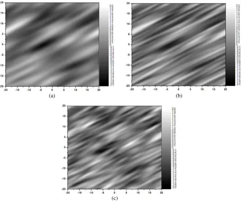
The size of the simulated rough surface is 40×40 m, and there are 1024 sampling points inx andy
directions. The simulated results are shown in Figure 1. Among them, (a) shows the simulation result, in which the RMS heightσ is 0.6 m, correlation length lx 10 m, ly 2 m and texture angleφ 30◦. Based
on the above parameters, (b) changes ly into 1 m, and (c) changes lx into 5 m and ly into 1 m. From
Figure 1, we clearly find that the textures from (b) become narrower than that from (c), and the height variations from (c) become much more obvious than that from (b).
3. SCATTERING THEORY FROM ROUGH SURFACE BY SSA
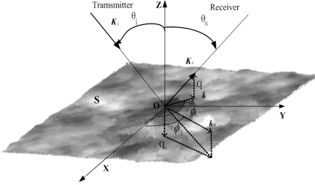
In SSA, the geometrical configuration adopted to resolve the wave-scattering problem from the 2-D randomly rough surface is illustrated in Figure 2, where we consider a rough interface z =h(r), with
r = (x, y), between two homogenous half-spaces with permittivity ε1 (upper half-space, z >0) and ε2
(lower half-space, z < 0) [26, 27]. The time dependence is assumed to be exp(−iωt). θi and θs are, respectively, incident and scattering elevation angles, and φi and φs are the incident and scattering azimuth angles, respectively. The incident wave vector can be expressed as Ki = k0−q0zˆ, where
k0
and −q0 are horizontal and vertical projections of the incident wave vector, respectively. The scattered
wave vector is Ks =k+qzˆ, where k and q are appropriate components of the scattered wave vector, respectively. q0 and q can be expressed as q0 =
ω2/c2−k2 0,q=
ω2/c2−k2, Imq
0,q ≥0 [28].
The unit vector in the direction of incidence is: ˆ
Ki = sinθicosφixˆ+ sinθisinφiyˆ−cosθizˆ (16)
and the incident wave vectorKi =KiKiˆ = (k0,−q0). The incident field can be expressed as:
ψinc(R) = exp
−iKi ·R
= exp
i(k0·r −iq0z)
= exp [−iKi(zcosθi−xsinθicosφi−ysinθisinφi)] (17)
where R = (r , q0) = (x, y, z) and ψinc is electric field E or magnetic field H depending on the
polarization.
The unit vector in the direction of scattering is:
ˆ
Ks = sinθscosφsxˆ+ sinθssinφsyˆ+ cosθszˆ (18)
and the scattered wave vector is Ks=KsKˆs= (
k , q). The scattered field can be expressed as:
ψsc(x, y, z) = exp
ik·r +iqz
S
k,k0
dk (19)
Considering the case of far-field approximation, the scattering amplitude matrix corresponding to the SSA method can be modified as
S
k,k0
= 2(qq0)
1/2
√
Pinc(q+q0)
dr
(2π)2 exp
−i
k−k0
·
r +i(q+q0)h(r)
×
B
k,k0
− i
4 M
k,k0, ξ ˆ h ξ exp
iξ·r
dξ
(20)
where B(k ,k0) is responsible for the first order contribution, and the following integration for the
second-order contribution. Moreover,Pincis the incident wave power received by the rough surface and can be expressed as:
Pinc=
|ψinc(x, y,0)|2dxdy (21)
and
M
k,k0,
ξ
= B2
k,k0, k−ξ
+B2
k,k0,
k0+ ξ
+ 2(q+q0)B
k,k0
(22) ˆ h ξ
= h(r) exp
−iξ ·r
dr (23)
where S =
S11 S12 S21 S22
, B =
B11 B12 B21 B22
, M =
M11 M12 M21 M22
, B2 =
B11(2) B (2) 12
B21(2) B (2) 22
which
describe mutual transformations of the EM waves of different polarizations. They are discussed in detail in [29]. Moreover, subscripts “1” and “2” denote vertical and horizontal polarizations, respectively. The left-hand number represents the polarization mode of the receiving antenna, and the right-hand number represents that of the transmitting antenna. Superscript “2” denotes second-order Bragg’ s kernel. For convenience, this paper only discusses co-polarizations HH andV V.
It can be confirmed that, in a general case,M(k,k0; 0) = 0. In view of this, the term related to the
functionM in Eq. (20) is proportional to the slopes of roughness rather than to the heights. This term provides a correction to SSA-I. In this paper, this term is realized through inverse Fourier transform to reduce the computational time.
Let us set
b11
k,k0;ε1, ε2
= (ε2−ε1)
ε1q(2)k +ε2qk(1)
−1
ε1q0(2)+ε2q(1)0
−1
(24)
b22
k,k0;ε1, ε2
= (ε2−ε1)
qk(2)+q(1)k
−1
q0(2)+q (1) 0
−1
where
qk(1) =
ε1ω 2
c2 −k2, q (2)
k =
ε2ω 2
c2 −k2
q0(1) =
ε1ω 2
c2 −k 2 0, q
(2) 0 =
ε2ω 2
c2 −k 2 0 (26) Then B11
k,k0
= b11
k,k0;ε1, ε2 ε1qk(2)q0(2) k·k0
kk0 −ε2kk0
(27)
B22
k,k0
= −b22
k,k0;ε1, ε2
ω2 c2
k·k0
kk0
(28)
B11(2)
k,k0; ξ;ε1, ε2
= b11
k,k0;ε1, ε2 −2 ε2−ε1 ε1q
(2)
ξ +ε2q
(1) ξ
×
ε1q(2)k q(2)0 k·ξ
k
ξ ·k0 k0
+ε2kk0ξ2
+2ε1ε2
q(1)ξ +qξ(2)
ε1q (2)
ξ +ε2q
(1) ξ
×
k0qk(2) k·ξ
k +kq (2) 0
ξ ·k0
k0
−ε1
Ks2q(2)k +Ks2q(2)0 + 2q (2)
k q(2)0
qξ(1)−qξ(2)
k·k0 kk0
(29)
B22(2)
k,k0; ξ;ε1, ε2
= b22
k,k0;ε1, ε2
ω2 c2
−2 ε2−ε1
ε1qξ(2)+ε2q(1)ξ
×
k·ξ k
ξ ·k0
k0 −ξ 2
k·k0
kk0
+
q(2)k +q(2)0 + 2
qξ(1)−qξ(2)
k·k0 kk0
(30)
Here, we choose medium 1 as air and medium 2 as general dielectric rough surface which means that the complex relative permittivity of the air is ε1 = (1,0), and that of medium 2 is calculated by
using Debye formulas [30].
In terms of rough surface scattering amplitudes calculated by the SSA-II method, the NRCS can be obtained by
σ0pq = 4πqq0ΔSpq
k,k0 ΔSpq
k,k0
∗
(31)
where
ΔSpq
k,k0
=Spq
k,k0
−Spq
k,k0
(32)
Expression (31) represents the scattered field corresponding to single rough surface, and subscript
pqdenotes polarization state. Due to the random characteristics of the rough surface, the final bistatic NRCS and backscattering coefficient are calculated as an average, i.e.,
σ0
pq =σpq0 (33)
4. NUMERICAL RESULTS AND ANALYSIS
4.1. Comparison of NRCS between SSA-I and SSA-II
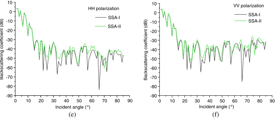
The single bistatic and backscattering NRCS versus angles from the rough surface for the texture angle of 0◦ is shown in Figure 3. Among them, (a) and (b) represent the bistatic scattering for the incident angle of 45◦. (c) and (d) represent that for the incident angle of 0◦. (e) and (f) represent the backscattering coefficient versus incident angles.
From Figure 3(a)–Figure 3(d), it is seen that for bistatic case, the NRCS from the SSA-II method is slightly larger than the SSA-I method for scattering angles departing from specular directions. For incident angleθi = 45◦, the distinction mainly appears at negative scattering angles, whereas forθi= 0◦, difference exists for both backward and forward directions. However, near the specular direction, such differences for both methods are very minor.
From Figure 3(e) and Figure 3(f), it is seen that for the backscattering case, in the quasi-specular region, the backscattering coefficients for both methods are almost the same, but as the incident angle increases, the coefficient for the SSA-II method is larger than that for the SSA-I method.
It is worthy to point out that the SSA-II method spends more computational time than the SSA-I method, but calculation accuracy of the SSA-II method is obviously higher than that of the SSA-I method. So this paper adopts the SSA-II method to study the scattering characteristics of the rough surface with different textures.
-90-80-70-60-50-40-30-20-10 0 10 20 30 40 50 60 70 80 90 -100
-90 -80 -70 -60 -50 -40 -30 -20 -10 0
10 HH polorization
Bistatic NRCS (dB)
SSA-I
Scattering angle ( ) SSA-II
-80 -70 -60 -50 -40 -30 -20 -10 0 10
Bistatic NRCS (dB)
VV polorization
SSA-I SSA-II
-80 -70 -60 -50 -40 -30 -20 -10 0
10 HH polorization
Bistatic NRCS (dB)
SSA-I
SSA-II
-80 -70 -60 -50 -40 -30 -20 -10 0 10
Bistatic NRCS (dB)
VV polorization
SSA-I SSA-II
o
-90-80-70-60-50-40-30-20-10 0 10 20 30 40 50 60 70 80 90 Scattering angle ( )o
-90-80-70-60-50-40-30-20-10 0 10 20 30 40 50 60 70 80 90 Scattering angle ( )o
-90-80-70-60-50-40-30-20-10 0 10 20 30 40 50 60 70 80 90 Scattering angle ( )o
(a) (b)
0 10 20 30 40 50 60 70 80 90 -90
-80 -70 -60 -50 -40 -30 -20 -10 0 10
Backscattering coefficient (dB)
SSA-I HH polarization
SSA-II
0 10 20 30 40 50 60 70 80 90
-90 -80 -70 -60 -50 -40 -30 -20 -10 0
10 VV polarization
Backscattering coefficient (dB)
SSA-I SSA-II
Incident angle ( )o
(e) (f)
Incident angle ( )o
Figure 3. Co-polarization scattering from a single rough surface: (a)–(d) show the variation of bistatic coefficients with scattering angles. (e) and (f) give the dependence of backscattering coefficients on incident angles. And black lines represent SSA-I and green lines represent SSA-II.
4.2. Comparison of Average NRCS for Rough Surface with Different Textures by SSA-II
The average bistatic and backscattering NRCS versus angles from the rough surface with different texture angles in SSA-II is shown in Figure 4. Among them, (a) and (b) represent the bistatic NRCS for the incident angle of 45◦, and (c) and (d) represent the backscattering coefficients.
From Figure 4(a) and Figure 4(b), it is seen that for bistatic case, as the texture angles increases from 0◦ to 90◦, the NRCS from the large texture angle is significantly larger than that from the small one for scattering angles departing from specular directions. However, near the specular direction, such differences for different texture angles are very minor. In addition, it is worthy to point out that for the texture angle of 90◦, the NRCS near the backward region significantly increases, especially in V V
polarization. This is because the incident plane is perpendicular to the texture direction, and more scattering facets contribute to the backward region.
From Figure 4(c) and Figure 4(d), it is seen that, for the backscattering case, in the quasi-specular region, the backscattering coefficients for different texture angles are almost the same, but as the incident angle increases, the coefficient for the large texture angle is larger than that for the small one.
-60 -50 -40 -30 -20 -10 0 10
-55 -50 -45 -35 -25 -15 -5 0 5
10 HH polarization
Average bistatic NRCS (dB)
-60 -50 -40 -30 -20 -10 0 10
-55 -45 -35 -25 -15 -5 5
VV polarization
Average bistatic NRCS (dB)
(a) (b)
-90-80-70-60-50-40-30-20-10 0 10 20 30 40 50 60 70 80 90 Scattering angle ( )o
-90-80-70-60-50-40-30-20-10 0 10 20 30 40 50 60 70 80 90 Scattering angle ( )o
o
φ = 45
φ = 90
φ = 0
o
o
o
φ = 45
φ = 90
φ = 0
o
-60 -50 -40 -30 -20 -10 0 10
-55 -45 -35 -25 -15 -5
5 HH polarization
Average ackscattering coefficient (dB)
-60 -50 -40 -30 -20 -10 0 10
-55 -45 -35 -25 -15 -5
5 VV polarization
Average ackscattering coefficient (dB)
(c) (d)
o
φ = 45 φ = 90 φ = 0
o
o
o
φ = 45 φ = 90 φ = 0
o
o
0 10 20 30 40 50 60 70 80 90
Incident angle ( )o
0 10 20 30 40 50 60 70 80 90
Incident angle ( )o
Figure 4. Average co-polarization scattering with different texture angles, i.e., φ = 0◦,45◦,90◦: (a) and (b) show the variation of bistatic coefficients with scattering angles. (c) and (d) give the dependence of backscattering coefficients on incident angles.
4.3. Effects of Statistical Parameters on Average Backscattering Coefficients
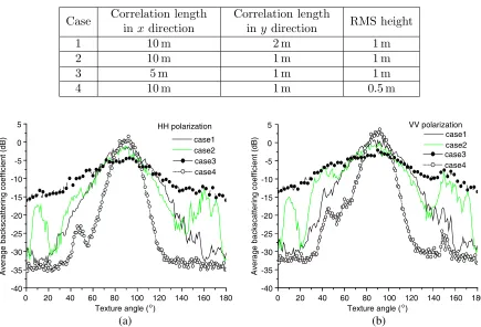
In the following, we merely choose the incident angle of 30◦. According to different correlation lengths and RMS heights, the calculations are divided into four groups which are shown in Table 1.
Table 1. Statistical parameters of different textures.
Case Correlation length inx direction
Correlation length
iny direction RMS height
1 10 m 2 m 1 m
2 10 m 1 m 1 m
3 5 m 1 m 1 m
4 10 m 1 m 0.5 m
0 20 40 60 80 100 120 140 160 180 -40
-35 -30 -25 -20 -15 -10 -5 0
5 HH polarization
case1 case2
Average backscattering coefficient (dB)
case3 case4
-40 -35 -30 -25 -20 -15 -10 -5 0
5 VV polarization
case1 case2
Average backscattering coefficient (dB)
case3 case4
(a) (b) Texture angle ( )o
0 20 40 60 80 100 120 140 160 180 Texture angle ( )o
The calculated results are shown in Figure 5. It is seen that for the texture angle of 90◦, the backscattering coefficients in any case are basically maximum and begin to reduce gradually for the texture angles departing from 90◦.
Comparing case 2 with case 4, we find that the backscattering coefficients from case 2 are significantly greater than that from case 4 except specular part. This is mainly because the RMS height of case 2 is two times greater than that of case 4. Namely, the texture surface corresponding to case 2 is much rougher than that of case 4. Moreover, comparing case 1 with case 3, under the condition that the ratio of correlation length lx to ly is 5 to 1 for both cases, the backscattering coefficients from case
3 is far larger than that from case 1 except specular part, which fully illustrates that small correlation length has a significant impact on the backscattering.
It is worthy to point out that because the SSA-II method is related to the slope of surface height, the backscattering coefficients are not strictly symmetric about the texture angle of 90◦, which is different from the results of the SSA-I method.
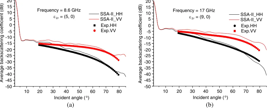
4.4. Comparisons of Experimental Data with Results Calculated by SSA-II
The average backscattering coefficients calculated by the SSA-II method are compared with the experimental data from asphalt surface in the literature [31], (Ulaby et al., 1986, Chapter 21, Figure 21.8). Among them, the size of the exponent spectrum rough surface is Lx = Ly = 15λinc,
where λinc is the EM wavelength. The statistical parameters are lx = ly = 3.574 mm, σ = 1.404 mm. The calculated sample number is 100. The calculated results are shown in Figure 6. For Figure 6(a), the incident frequency is f = 8.6 GHz, and the relative permittivity of medium 2 isε2r = (5,0), while
for Figure 6(b), f = 17 GHz andε2r= (9,0).
10 20 30 40 50 60 70 80
Average backscattering coefficient (dB)
SSA-II_HH SSA-II_VV Frequency = 8.6 GHz
Exp.HH Exp.VV
Average backscattering coefficient (dB)
SSA-II_HH SSA-II_VV
Exp.HH Exp.VV
Incident angle ( )o
10 20 30 40 50 60 70 80
Incident angle ( )o
(a) (b)
20 15 10 5 0 -5 -10 -15 -20 -25 -30 -35 -40 -45 -50
20 15 10 5 0 -5 -10 -15 -20 -25 -30 -35 -40 -45 -50
ε 2r= (5, 0)
Frequency = 17 GHz
ε 2r= (9, 0)
Figure 6. Comparison of results by the SSA-II method and measured data of an asphalt surface at (a) 8.6 GHz and (b) 17 GHz, respectively.
5. CONCLUSION
In this paper, the SSA-II method is applied to calculate the scattering from 2-D randomly Gaussian rough dielectric surfaces for different texture models. A comparative study has been done on the distinct properties of both NRCS due to texture effects among waves. From the numerical results of bistatic and backscattering NRCS, it is seen that the differences between the SSA-I and SSA-II methods are revealed, and the effects of statistical parameters and texture angle on the scattering are further analyzed. In summary, the analysis presented in this paper helps to establish better understanding of the scattering features of the 2-D texture rough surface. Meanwhile, this paper provides important reference value for the texture information of 2-D rough surface. It is worthy to point out that the numerical scattering results of texture rough surfaces remain to be further verified through measurement data.
ACKNOWLEDGMENT
The authors would like to thank the Fundamental Research Funds for the Central Universities, the National Natural Science Foundation of China, and the Aerospace Research Institute of Materials and Processing Technology for the support to this research.
REFERENCES
1. Tsang, L. and J. A. Kong, Scattering of Electromagnetic Waves, Advanced Topics, Wiley Series in Remote Sensing, Wiley Interscience, New York, 2001.
2. Zhao, Y. W., M. Zhang, X. Geng, and P. Zhou, “A comprehensive facet model for bistatic SAR imagery of dynamic ocean scene,”Progress In Electromagnetics Research, Vol. 123, 427–445, 2012. 3. Mcdaniel, S. T., “An extension of the small-slope approximation for rough surface scattering,”
Waves in Random Media, Vol. 5, No. 2, 201–214, 1995.
4. Sun, R. Q., G. Luo, M. Zhang, and C. Wang, “Electromagnetic scattering model of the Kelvin wake and turbulent wake by a moving ship,” Waves in Random Media, Vol. 21, No. 3, 501–504, 2011.
5. Chen, H., M. Zhang, and H.-C. Yin, “Facet-based treatment on microwave bistatic scattering of three-dimensional sea surface with electrically large ship,”Progress In Electromagnetics Research, Vol. 123, 385–405, 2012.
6. Warnick, K. F. and W. C. Chew, “Numerical simulation methods for rough surface scattering,”
Waves in Random Media, Vol. 11, No. 1, R1–R30, 2001.
7. Thorsos, E. I., “The validity of the Kirchhoff approximation for rough surface scattering using a Gaussian roughness spectrum,”J. Acoust. Soc. Am., Vol. 83, No. 1, 78–92, 1988.
8. Guo, L.-X., Y. Liang, J. Li, and Z.-S. Wu, “A high order integral SPM for the conducting rough surface scattering with the tapered wave incidence — TE case,” Progress In Electromagnetics Research, Vol. 114, 333–352, 2011.
9. Lee, P. H. Y., et al., “Wind-speed dependence of small-grazing-angle microwave backscatter from sea surfaces,” IEEE Trans. Antennas Propagat., Vol. 44, No. 3, 333–340, 1996.
10. Sajjad, N., A. Khenchaf, et al., “An improved two-scale model for the ocean surface bistatic scattering,” Proc. Of International Geoscience and Remote Sensing Symposium, Vol. 1, 387–390, 2008.
11. Vaitilingom, L. and A. Khenchaf, “Radar cross sections of sea and ground clutter estimated by two scale model and small slope approximation in Hf-VHF bands,” Progress In Electromagnetics Research B, Vol. 29, 311–338, 2011.
12. Voronovich, A. G., “Small-slope approximation in wave scattering by rough surfaces,” Sov. Phys.-JETP, Vol. 62, 65–70, 1985.
14. Toporkov, J. V. and G. S. Brown, “Numerical study of the extended Kirchhoff approach and the lowest order small slope approximation for scattering from ocean-like surfaces: Doppler analysis,”
IEEE Trans. Antennas Propagat., Vol. 50, No. 4, 417–425, 2002.
15. Chevalier, B. and G. Berginc, “Small-slope approximation method: scattering of a vector wave from 2-D dielectric and metallic surfaces with Gaussian and non-Gaussian statistics,” Proceedings of SPIE, Vol. 4100, 22–32, 2000.
16. Johnson, J. T. and K. F. Warnick, “On the geometrical optics (Hagfors’ law) and physical optics approximations for scattering from exponentially correlated surfaces,”IEEE Trans. Geosci. Remote Sens., Vol. 45, No. 8, 2619–2629, 2007.
17. Hu, S. Z., et al., “Comparison of various approximation theories for randomly rough surface scattering,”Wave Motion, Vol. 46, No. 5, 281–292, 2009.
18. Li, X. F. and X. J. Xu, “Scattering and doppler spectral analysis for two-dimensional linear and nonlinear sea surfaces,”IEEE Trans. Geosci. Remote Sens., Vol. 49, No. 2, 603–611, 2011.
19. Cao, G. Z., P. Hou, Y. Q. Jin, et al., “Image fusion of SAR remote sensing with Laplacian Pyramid transformation fusion algorithm based on local conditional information of image,”Remote Sensing Technology and Application, Vol. 22, No. 5, 628–632, 2007.
20. Wei, P. B., M. Zhang, R. Q. Sun, and X. F. Yuan, “Scattering studies for two-dimensional exponential correlation textured rough surfaces using small-slope approximation method,” IEEE Trans. Geosci. Remote Sens., Vol. 52, No. 9, 5364–5373, 2014.
21. Prakash, R., D. Singh, and N. P. Pathak, “Microwave specular scattering response of soil texture at X-band,”Advances in Space Research, Vol. 44, No. 7, 801–814, 2009.
22. Hu, Y. Z. and K. Tonder, “Simulation of 3-D random rough surface by 2-D digital filter and Fourier analysis,”Int. J. Mach. Tools Manufact., Vol. 32, No. 12, 83–90, 1992.
23. Zhang, M., H. Chen, and H. C. Yin, “Facet-based investigation on EM scattering from electrically large sea surface with two-scale profiles: Theoretical model,” IEEE Trans. Geosci. Remote Sens., Vol. 49, No. 6, 1967–1975, 2011.
24. Tsang, L., J. A. Kong, K. H. Ding, and C. A. Ao,Scattering of Electromagnetic Waves, Numerical Simulations, 124–134, Wiley Series in Remote Sensing, Wiley Interscience, New York, 2001. 25. Tatarskii, V. I. and V. V. Tatarskii, “Statistical non-Gaussian model of sea surface with anisotropic
spectrum for wave scattering theory. Part I,” Progress In Electromagnetics Research, Vol. 22, 259– 291, 1999.
26. Voronovich, A. G. and V. U. Zavorotny, “Theoretical model for scattering of radar signals in Ku-and C-bKu-ands from a rough sea surface with breaking waves,” Waves in Random Media, Vol. 11, No. 3, 247–269, 2001.
27. Voronovich, A. G., “Small-slope approximation for electromagnetic wave scattering at a rough interface of two dielectric half-spaces,”Waves in Random Media, Vol. 4, 337–367, 1994.
28. Chevalier, B. and G. Berginc, “Small-slope approximation method: scattering of a vector wave from 2-D dielectric and metallic surfaces with Gaussian and non-Gaussian statistics,” Proceedings of SPIE, Vol. 4100, 22–32, 2000.
29. Bourlier, C., N. D´echamps, and G. Berginc, “Comparison of asymptotic backscattering models (SSA, WCA, and LCA) from one-dimensional Gaussian ocean-like surfaces,”IEEE Trans. Antennas Propagat., Vol. 53, No. 5, 1640–1652, 2005.
30. Stogryn, A., “Equations for calculating the dielectric constant of saline water,”IEEE Trans. Micro. Theory Tech., Vol. 19, No. 8, 733–736, 1971.