Neural Models for the Elliptic- and Circular-Shaped Microshield Lines

NEURAL MODELS FOR THE ELLIPTIC- AND CIRCULAR-SHAPED MICROSHIELD LINES

S. Kaya, M. Turkmen, K. Guney, and C. Yildiz

Department of Electrical and Electronics Engineering Faculty of Engineering

Erciyes University 38039, Kayseri, Turkey

Abstract—This article presents a new approach based on artificial neural networks (ANNs) to calculate the characteristic parameters of elliptic and circular-shaped microshield lines. Six learning algorithms, bayesian regularization (BR), Levenberg-Marquardt (LM), quasi-Newton (QN), scaled conjugate gradient (SCG), resilient propagation (RP), and conjugate gradient of Fletcher-Reeves (CGF), are used to train the ANNs. The neural results are in very good agreement with the results reported elsewhere. When the performances of neural models are compared with each other, the best and worst results are obtained from the ANNs trained by the BR and CGF algorithms, respectively.

1. INTRODUCTION

In recent years, microshield lines have aroused great interest in microwave integrated circuit (MIC) and monolithic MIC (MMIC) applications [1–10]. The microshield lines, comparing with the conventional ones such as the microstrip or the coplanar waveguide, have the ability to operate without the need for via-holes or the use of air bridges for ground equalization. Further advantages include low radiation loss, reduced electromagnetic interference, the availability of a wide range of impedances, and compatibility with antennas of microstrip or aperture type.

The characteristic impedances for V, elliptic, and circular-shaped microshield lines were derived by using CMT [4]. The CMT has also been used to determine the quasi-TEM characteristic parameters of microshield lines with practical cavity sidewall profiles [5]. The closed form formulas have been developed for the evaluation of the quasi-TEM characteristic parameters of asymmetrical V-shaped microshield line [6]. A generalized potential-matching technique has been developed to calculate the capacitance and characteristic impedance of microshield lines enclosed by shields of arbitrary shape [7]. The finite-element analysis of generalized V- and W-shaped shielded microstrip lines in an anisotropic medium has been proposed in 2001 [8]. The field patterns of the dominant mode and the first higher-order mode in the V-shaped microshield line were calculated by using the edge-based finite-element method [9]. The even- and odd-mode characteristic impedances and the effective permittivities of a membrane supported air-filled V-groove coupled microshield line have been calculated using finite element method [10]. The methods proposed in the literature [1– 10] for the analysis of microshield structures have been used with their own benefits and limitations.

In this paper, an alternative method based on artificial neural networks (ANNs) is used to compute accurately the characteristic parameters of the elliptic-shaped microshield lines (ESMLs) and the circular-shaped microshield line (CSMLs). ANNs are being increasingly used in the analysis and design of microwave devices and circuits due to their ability and adaptability to learn, generalizability, smaller information requirement, fast real-time operation, and ease of implementation features [11–17]. Because of these attractive features, in this paper, neural models are presented for calculating the characteristic parameters of the ESML and the CSML. First, the parameters of the ESML and CSML related to the characteristic parameters are determined, and then the effective permittivity and characteristic impedance depending on these parameters are calculated by using the neural models. Six learning algorithms, BR [18], LM [19], QN [20], SCG [21], RP [22], and CGF [23], are used to train the neural models. These learning algorithms are employed to obtain better performance and faster convergence with simpler structure. The characteristic parameters obtained by using neural models are in very good agreement with the results available in the literature.

is explained. The results are then presented and conclusion is made.

(a)

(b)

h2

h1

S=2a

W W

2b

r 0

h2=b

h1

S=2a

W W

2b

0

r ε

ε

ε

ε

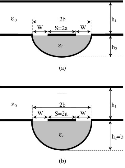
Figure 1. Microshield lines, (a) ESML and (b) CMSL.

2. CHARACTERISTIC PARAMETERS OF ESML AND CSML

The cross-sections of ESML and CSML with upper shielding are shown in Figs. 1(a) and (b). The center conductor, of widthS = 2a, is placed between the two ground planes, of spacing 2b, which are located on a substrate of thickness h2, with relative permittivity εr. It is noted

that the CSML is a special case of the ESML whenh2 =b. The total

capacitance for an ESML is given in [4]

CT(εr) =C1+C2 (1)

where

C1 = 2·ε0·

K(k1)

whereK(k1) and K(k1) are the complete elliptic integrals of the first

kind with the modulus of k1 and k1. k1 is a complementary modulus

ofk1 and equals to (1−k12)1/2. The modulusk1 is defined in terms of

geometrical dimensions of microshield line as in reference [4]:

k1 =

tanh

π·S

4·h1

tanh

π·(S+ 2·W)

4·h1

(3)

C2 = π·ε0·εr·

lnb+h2

a + ln

1−B −1

(4) with

B =

b2_−h2 2−a

2

(b−h2)

2h2a

(5) The effective permittivity and characteristic impedance of ESML are given as

εeff =

CT (εr)

CT(1) (6)

Z0 =

1

c· √εeff ·CT(1)

(7)

wherecis the velocity of light in vacuum andCT(1) is the capacitance

when replacing the dielectric substrate by air.

3. ARTIFICIAL NEURAL NETWORKS (ANNs)

ANN learns relationships among sets of input-output data which are characteristic of the device under consideration. It is a very powerful approach for building complex and nonlinear relationship between a set of input and output data. ANNs are developed from neurophysiology by morphologically and computationally mimicking human brains [11, 12, 24]. Although the precise operation details of ANNs are quite different from those of human brains, they are similar in three aspects: they consist of a very large number of processing elements (the neurons), each neuron connects to a large number of other neurons, and the functionality of networks is determined by modifying the strengths of connections during a learning phase.

factors. ANNs have many structures and architectures [11, 12, 24]. The class of ANN and/or architecture selected for a particular model implementation depends on the problem to be solved. After several experiments using different architectures coupled with different training algorithms, in this paper, the MLP neural network architecture [24] was used to compute the characteristic parameters of ESMLs and CSMLs.

The MLP is one of the most extensively used ANN, due to well-known general approximation capabilities, despite its limited complexity. The MLP comprises an input layer, an output layer, and a number of hidden layers. Neurons in the input layer only act as buffers for distributing the input signals xi to neurons in the hidden

layer. Each neuron j in the hidden layer sums up its input signals xi

after weighting them with the strengths of the respective connections

wji from the input layer and computes its outputyj as a functionf of

the sum, namely

yj =f wjixi

(8)

f can be a simple threshold function, a sigmoidal or hyperbolic tangent function. The output of neurons in the output layer is computed similarly.

Training a network consists of adjusting weights of the network using a learning algorithm. The learning algorithm gives the change ∆wji(k) in the weight of a connection between neuronsiandjat time k. The weights are then updated according to the following formula:

wji(k+ 1) =wji(k) + ∆wji(k+ 1) (9)

MLPs can be trained using many different learning algorithms [24]. In this article, the following six learning algorithms described briefly were used to train the MLPs:

3.1. Bayesian Regularization (BR) Algorithm

The BR algorithm updates the weight and bias values according to the LM optimization and minimizes a linear combination of squared errors and weights [18]. It also modifies the linear combination so that at the end of training the resulting network has good generalization qualities. Backpropagation is used to compute the Jacobian JX of performance with respect to the weight and bias variables X. Each variable is adjusted according to LM:

3.2. Levenberg-Marquardt (LM) Algorithm

The LM algorithm is a least-squares estimation algorithm based on the maximum neighborhood idea [19]. The objective error functionE(w) can be written as

E(w) =

m

i=1

e2_i(w) =g(w)2 (11)

with

e2_i(w) = (ydi−yi)2 (12)

where g(w) is a function containing the individual error terms, ydi is

the desired value of output neuron i, and yi is the actual output of that neuron.

It is assumed that function g(w) and its Jacobian J are known at point w. The LM algorithm is used to compute the weight vector

w such that E(w) is minimum. A new weight vector wk+1 can be

obtained from the previous weight vectorwk as follows:

wk+1 =wk+δwk (13)

with

δwk=− JkTg(wk)

J_kTJk+λI

₋1

(14) where k is the number of the iterations, Jk is the Jacobian of g(wk)

evaluated by taking derivative of g(wk) with respect to wk, λ is the

Marquardt parameter, andI is the identity matrix. 3.3. Quasi-Newton (QN) Algorithm

The basic QN algorithm consists of the following steps [20]: I. set a search direction sk =−Hk·gk,

II. wk+1 =wk+η·sk,

III. update Hk giving Hk+1

whereH is the approximate inverse second derivative matrix,g is the first derivative term, η is a scalar step length parameter, and s is a updating direction. The major concept of the algorithm is the updating strategy for the approximate inverse second derivative matrix. Hk+1

is evaluated by using the following formula:

Hk+1=H+

1 +γ

T_Hγ

σT_γ

σσT

σT_γ −

σγTH+HγσT

with

γk=gk+1−gk (16)

and

σk=ηsk=wk+1−wk (17)

The initial matrixH is usually selected to be a unit matrix. 3.4. Scaled Conjugate Gradient (SCG) Algorithm

The SCG algorithm [21] is an implementation of avoiding the complicated line search procedure of conventional conjugate gradient algorithm. For the SCG algorithm, the Hessian matrix is approximated by using the following formula

E(wk)sk ≈ E

_{(wk+σksk)−E(wk)} σk

+λksk (18) where E and E are the first and second derivative information of error function E(wk). The other terms sk, σk and λk represent the

search direction, the parameter controlling the change in weight for second derivative approximation, and the parameter for regulating the indefiniteness of the Hessian, respectively. In order to get a good quadratic approximation of E, a mechanism to raise and lower λk is

needed when the Hessian is positive definite [21]. 3.5. Resilient Propagation (RP) Algorithm

The RP algorithm determines the direction of the weight update by using the sign of the derivative and determines the size of the weight change by a separate update value. For each weight, the adaptive individual update value ∆ij evolves during the learning process based

on its local sight on the error function, E, according to the following learning-rule [22].

∆ij(k) =

      

η+_·∆

ij(k−1), if ∂E_∂w(k_ij−1) ·∂E_∂w(_ijk) >0

η−·∆ij(k−1), if ∂E_∂w(k−1)

ij ·

∂E(k)

∂wij <0

∆ij(k−1), otherwise

(19)

where 0 < η− < 1 < η+_{. The weights are updated by using the}

following formula:

∆wij(k) =       

−∆ij(k), if ∂E_∂w(_ijk) >0

+∆ij(k), if ∂E_∂w(k)

ij <0

0, otherwise

3.6. Conjugate Gradient of Fletcher-Reeves (CGF) Algorithm

The CGF algorithm updates weight and bias values according to the formulas proposed by Fletcher-Reeves [23]. The method of conjugate directions can be used to minimize a positive definite quadratic function in n steps. The minimum of E is found by a sequence of linear searches along directionssk,k= 1,2, . . . , n

wk+1 =wk+µksk (21)

with

µk= arg min_µ E(wk+µsk) (22)

and

sk+1 =−d(wk+1) +βksk (23)

whered(wk) = ∂E_∂w(w_ij)

w=wk

, and βk is given by [23]:

βk=

d(wk+1)Td(wk+1)

d(wk)Td(wk)

(24)

4. ANNs FOR CHARACTERISTIC PARAMETERS

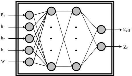
In this paper, the neural models are used for calculating the characteristic parameters of ESML and CSML. For the neural models, the inputs areεr,h1,h2, b, and W, and the outputs are the effective

permittivity (εeff) and the characteristic impedance (Z0). A neural

model used in calculating the characteristic parameters of ESML and CSML is shown in Fig. 2. Only one neural model is used to calculate the characteristic parameters of both ESML and CSML with different electrical properties and different geometrical dimensions.

ANN models are a kind of black box models, whose accuracy depends on the data presented to it during training. A good collection of the training data, i.e., data which is well-distributed, sufficient, and accurately simulated, is the basic requirement to obtain an accurate model. For microwave applications, there are two types of data generators, namely measurement and simulation. The selection of a data generator depends on the application and the availability of the data generator. The training data sets used in this paper were obtained from the method proposed by Yuan et al. [4]. 28380 data sets were used to train the neural models. Training data sets are in the range of 2 ≤ εr ≤ 19, 1 mm ≤ h1 ≤ 5.5 mm, 200µm ≤ h2 ≤ 1200µm,

r

eff h2

h1

b

W

Z0 ε ε

Figure 2. ANN structure for ESMLs and CSMLs.

which are completely different from training data sets, were used to test the ANNs.

Training the ANNs with the use of a learning algorithm to calculate the characteristic parameters of the ESMLs and the CSMLs involves presenting them sequentially and/or randomly with different sets (εr,h1,h2, b, andW) and corresponding characteristic parameters

(εeff and Z0). First, the input vectors (εr, h1, h2, b, and W) are

presented to the input neurons and output vectors (εeff and Z0) are

computed. ANN outputs are then compared to the known outputs of the training data sets and errors are computed. Error derivatives are then calculated and summed up for each weight until all the training examples have been presented to the network. These error derivatives are then used to update the weights for neurons in the model. Training proceeds until errors are lower than prescribed values.

5. NUMERICAL RESULTS AND CONCLUSION

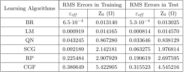
In this study, the characteristic parameters of ESMLs and CSMLs are computed with the use of neural models. The training and test RMS errors of neural models are given in Table 1. When the performances of neural models are compared with each other, the best and worst results for training and test were obtained from the models trained with the BR and CGF algorithms, respectively, as shown in Table 1. Table 1. Training and test RMS errors of neural models.

Learning Algorithms RMS Errors in Training RMS Errors in Test

εeff Z0(Ω) εeff Z0 (Ω)

BR 6.5·10−4 _{0.013140 5.3·10}−4 _0.013025

LM 0.000919 0.014165 0.000814 0.014570

QN 0.043245 0.867280 0.033646 0.838129

SCG 0.092189 2.142181 0.063275 1.976814

RP 0.225484 2.907929 0.190619 2.697595

CGF 0.380649 5.422905 0.315523 4.545216

The effective permittivity and characteristic impedance test results of neural model trained by BR algorithm are compared with the results of CMT [4] in Figs. 3 and 4. The variation of the characteristic parameters with respect to the slot width (W) is shown in Fig. 3 for the ESMLs with with h1 = 3 mm, h2 = 400µm, b = 692.82µm,

and εr = 2.55, 3.78, 10, and 12.9. Fig. 4 illustrates the variation

of the characteristic parameters with respect to the slot width (W) for the CSMLs with h1 = 3 mm, h2 = 400µm, b = 400µm, and

εr = 2.55, 3.78, 10, and 12.9. It is clear from Figs. 3 and 4 that the

results of neural model for the effective permittivities and characteristic impedances of both ESML and CSMLs are in very good agreement with the results of CMT. This very good agreement supports the validity of neural model presented in this paper.

It should be emphasized that better results may be obtained from the neural models either by choosing different training and test data sets from the ones used in the paper or by supplying more input data set values for training. The high-speed real-time computation feature of the neural models recommends their use in MIC and MMIC CAD programs.

0 1 2 3 4 5 6 7 8 9 10

0 100 200 300 400 500 600 700 800

Slot width, W (µm)

Effective permittivity . 0 40 80 120 160 200

0 100 200 300 400 500 600 700 800 Slot width, W (µm)

Characteristic impedance ( ) . Ω (a) (b)

Figure 3. Comparison of the neural model and CMT [4] results for the characteristic parameters of ESMLs withh1 = 3 mm,h2 = 400µm,

b = 692.82µm, and εr = 2.55, 3.78, 10, and 12.9. (a) Effective permittivity and (b) Characteristic impedance.

Ω (a) (b) 0 1 2 3 4 5 6 7 8 9

0 50 100 150 200 250 300 350 400 Slot width, W (µm)

Effective permittivity . 0 20 40 60 80 100 120 140 160 180

0 50 100 150 200 250 300 350 400 Slot width, W (µm)

Characteristic impedance

(

)

.

Figure 4. Comparison of the neural model and CMT [4] results for the characteristic parameters of CSMLs withh1 = 3 mm,h2 = 400µm,

b = 400µm, and εr = 2.55, 3.78, 10, and 12.9. (a) Effective

performance and faster convergence with simpler structure. The best result is obtained from the MLPs trained by BR algorithm. The main advantage of the method proposed here is that only one neural model is used to calculate the characteristic parameters of both ESMLs and CSMLs. The method proposed here can easily be applied to other microwave problems.

REFERENCES

1. Dib, N. I., W. P. Harokopus, L. P. B. Katehi, C. C. Ling, and G. M. Rebeiz, “Study of a novel planar transmission line,” IEEE MTT-S Int. Microwave Symp. Dig., 623–626, Boston, 1991. 2. Dib, N. I. and L. P. B. Katehi, “Impedance calculation for the

microshield line,” IEEE Microwave Guided Wave Lett., Vol. 2, 406–408, 1992.

3. Schutt-Aine, J. E., “Static analysis of V transmission lines,”IEEE Trans. Microwave Theory Techniques, Vol. 40, 659–664, 1992. 4. Yuan, N., C. Ruan, and W. Lin, “Analytical analyses of V, elliptic,

and circular-shaped microshield transmission lines,”IEEE Trans. Microwave Theory Techniques, Vol. 42, 855–859, 1994.

5. Cheng, K. K. M. and I. D. Robertson, “Quasi-TEM study of microshield lines with practical cavity sidewall profiles,” IEEE Trans. Microwave Theory Techniques, Vol. 43, 2689–2694, 1995. 6. Cheng, K. K. M. and I. D. Robertson, “Simple and explicit

formulas for the design and analysis of asymmetrical V-shaped microshield line,” IEEE Trans. Microwave Theory Techniques, Vol. 43, 2501–2504, 1995.

7. Kiang, J. F., “Characteristic impedance of microshield lines with arbitrary shield cross section,” IEEE Trans. Microwave Theory Techniques, Vol. 46, 1328–1331, 1998.

8. Yan, Y. and P. Pramanick, “Finite-element analysis of generalized V- and W-shaped edge and broadside-edge-coupled shielded microstrip line on anisotropic medium,” IEEE Trans. Microwave Theory Techniques, Vol. 49, 1649–1657, 2001.

9. Lu, M. and P. J. Leonard, “Edge-based finite-element analysis of the field patterns in V-shaped microshield line,” Microwave and Optical Technology Letters, Vol. 41, 43–47, 2004.

11. Christodoulou, C. G. and M. Georgiopoulos,Application of Neural Networks In Electromagnetics, Artech House, MA, 2001.

12. Zhang, Q. J. and K. C. Gupta, Neural Networks for RF and Microwave Design, Artech House, 2000.

13. Guney, K., C. Yildiz, S. Kaya, and M. Turkmen, “Artificial neural networks for calculating the characteristic impedance of air-suspended trapezoidal and rectangular-shaped microshield lines,” Journal of Electromagnetic Waves and Applications, Vol. 20, 1161–1174, 2006.

14. Guney, K., C. Yildiz, S. Kaya, and M. Turkmen, “Neural models for the broadside-coupled V-shaped microshield coplanar waveguides,” International Journal of Infrared and Millimeter Waves, Vol. 27, 1241–1255, 2006.

15. Yildiz, C., K. Guney, M. Turkmen, and S. Kaya, “Neural models for coplanar strip line synthesis,” Progress In Electromagnetics Research, PIER 69, 127–144, 2007.

16. Guney, K., C. Yildiz, S. Kaya, and M. Turkmen, “Neural models for the V-shaped conductor-backed coplanar waveguides,” Microwave and Optical Technology Letters, Vol. 49, 1294–1299, 2007.

17. Yildiz, C., K. Guney, M. Turkmen, and S. Kaya, “Neural models for quasi-static analysis of conventional and supported coplanar waveguides,” AE ¨U International Journal of Electronics and Communications, Vol. 61, 521–527, 2007.

18. Mackay, D. J. C., “Bayesian interpolation,” Neural Computation, Vol. 4, 415–447, 1992.

19. Hagan, M. T. and M. Menjah, “Training feedforward networks with the Marquardt algorithm,” IEEE Transactions on Neural Networks, Vol. 5, 989–993, 1994.

20. Gill, P. E., W. Murray, and M. H. Wright,Practical Optimization, Academic Press, New York, 1981.

21. Moller, M. F., “A scaled conjugate gradient algorithm for fast supervised learning,” Neural Networks, Vol. 6, 525–533, 1993. 22. Reidmiller, M. and H. Braun, “A direct adaptive method for faster

backpropagation learning: The Rprop algorithm,”Proceedings of the IEEE Int. Conf. on Neural Networks, 586–591, San Francisco, 1993.

23. Fletcher, R. and C. M. Reeves, “Function minimization by conjugate gradients,”Comput. J., Vol. 7, 149–154, 1964.