Piston Modelling and Gas-Solid Mixing Characterization in JBR

(1)

Scholarship@Western

Electronic Thesis and Dissertation Repository

November 2018

Piston Modelling and Gas-Solid Mixing Characterization in JBR

Tian Dong Cai

The University of Western Ontario

Supervisor Briens, Cedric L.

The University of Western Ontario Joint Supervisor Berruti, Franco

The University of Western Ontario

Graduate Program in Chemical and Biochemical Engineering

A thesis submitted in partial fulfillment of the requirements for the degree in Master of Engineering Science

Follow this and additional works at: https://ir.lib.uwo.ca/etd

Part of the Chemical Engineering Commons

Recommended Citation Recommended Citation

Cai, Tian Dong, "Piston Modelling and Gas-Solid Mixing Characterization in JBR" (2018). Electronic Thesis and Dissertation Repository. 5774.

https://ir.lib.uwo.ca/etd/5774

This Dissertation/Thesis is brought to you for free and open access by Scholarship@Western. It has been accepted for inclusion in Electronic Thesis and Dissertation Repository by an authorized administrator of

(2)

The Jiggle Bed Reactor (JBR), a batch fluidized bed microreactor, is inexpensive and easy to operate with a small amount of solids. The main goal of this thesis was to provide practical tools for the design and operation of JBR systems that will ensure good gas-solids mixing.

A model was developed to predict the piston motion. The model uses four empirical parameters that change depending on the equipment characteristics. Two parameters characterize the gas supply to the piston and two parameters are used to describe the frictional forces on the piston. The model was validated with high speed video.

Experiments were conducted to study the effect of the reactor motion on the gas-solid mixing in the JBR. A good correlation between gas-solid mixing in the reactor and the maximum

acceleration of the piston was identified: good gas-solid mixing was achieved with maximum accelerations greater than 55 m/s2.

Keywords

(3)

ii

Co-Authorship Statement (where applicable)

(4)

iii

Acknowledgments

This research project would not have been possible without the generous support of numerous people. I would like to take this opportunity to thank my respected supervisors: Dr. C. Briens and Dr. F. Berruti for their guidance, encouragement and support despite all the hardships and

challenges throughout this project. I am thankful to Dr. Xiaotao (Tony), Bi for his kind referral and support for my application to UWO back in late 2015, and for the OGS in late 2016. I would have never dreamed to have such precious opportunities and privileges to work with experts like them in the field of particle fluidization.

I am also thankful to all my colleagues in the Institution for Chemicals from Alternative Resources (ICFAR). My special thanks go to the on-site technician Thomas Johnson who

devoted much of his work and talent to assist me building the solid vessel and post-doc fellow Dr. Francisco Javier Sanchez Careaga who kindly helped me developed the Arduino based control and DAQ program for the apparatus. Former post-doctoral fellow Stefano Tacchino devoted some of his precious time to help me learning how to conduct research when I first started my master program back in the summer of 2016. My good colleague Aaron Joness provided many valuable and creative advice and ideas for compiling the hardware configuration and MATLAB analytic scripts for this project. Mr. Pengzhi Mao, a visiting undergraduate student from the University of Tianjin also contributed greatly to the work on the piston modelling. Many of my other colleagues like Tracy Hu kindly provided me a lift to the institution during countless weekend shifts. Without their help, this thesis would have been much delayed. I wish them all best in their life and future career.

In particular, I would like to express my gratitude to Christine Ramsden and Chantal Gloor whom provided their best possible assistance on numerous administrative and financial services at ICFAR.

(5)

iv

I am also gratefully acknowledging the Chemical and Biochemical Engineering Department (CBE), School of Graduate and Postdoctoral Studies (SOGPS), the Society of Graduate Studies (SOGS), University Machine Services (UMS), Electronic Workshop, Information Technology Service (ITS) and Engineering Financial Store (EFS) for various assistances received throughout this master study.

(6)

v

List of Tables

Table 3-1 Input and output involved in virtual tube calculations. ... 21

Table 3-2 The seven cases of spool position and the resultant air passage situation within the valve. ... 33

Table 3-3 Input and output summary for the double solenoid valve model. ... 34

Table 3-4 Input and output summary for tube delay model. ... 42

Table 3-5 Values of ζ when fluid experiences sudden expansion. ... 47

Table 3-6 Values of ζ when fluid experiences sudden contraction. ... 47

Table 3-7 Summary table of terms and calculations involved in the four major parts. ... 57

Table 4-1 Averaged tube fill-up time... 75

Table 4-2 Summary of averaged chamber filling-up time under a given feed pressure. ... 75

Table 4-3 Summary of time needed to move to top at different pressure feed. ... 77

Table 4-4 Summary of time needed to move to bottom at different pressure feed. ... 78

Table 5-1 Cross comparison of piston motion parameters and CV values of a well-mixed case and a poorly-mixed case. ... 102

Table 5-2 Model predicted accelerations under given conditions meeting the minimum requirement. ... 110

Table D-1 Pressure transducer calibration data (raw) ... 189

(10)

ix

List of Figures

Figure 1-1 A schematic illustration of the JBR system developed earlier [Latifi et al., 2014]. ... 3

Figure 1-2 Sequences of mixing of solid particles in the JBR with bed expansion during

downward actuator retraction [Latifi et al., 2014]. ... 4

Figure 1-3 Sequences of mixing of solid particles in the JBR with bed contraction during upward actuator extension [Latifi et al., 2014]. ... 4

Figure 2-1 Overview of major components in the experimental apparatus: (a) high speed camera, (b) solid vessel, (c) Red LED, (d) Pneumatic Actuator, (e) Pressure Transducers, (f) Double solenoid Valve, (g) Control board with relays. ... 8

Figure 2-2 Transparent JBR vessel; note that its backside (along with the platform) is covered in black tape to make contrast with the white sand during JBR trials with the red LED wrapped in black showing only its tip (see the boxed region). ... 10

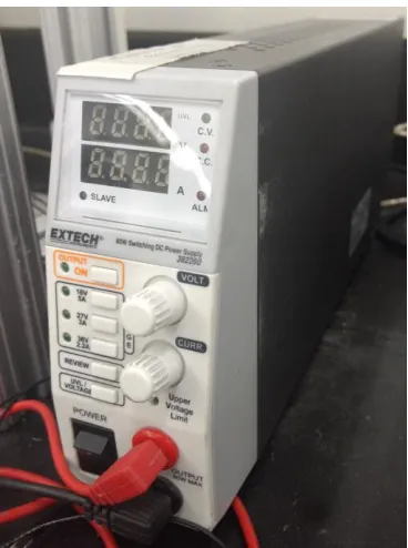
Figure 2-3 Signal generator used for powering the red LED. ... 10

Figure 2-4 Arduino based feedforward relay controller (from:

https://reactivesystems.wordpress.com/2012/02/11/pneumatic-actuators/ ). ... 12

Figure 2-5 METALWORK diaphragm air pressure regulator used for maintaining feed to the system. ... 13

Figure 2-6 Actual METALWORK 5/2 3/8 inch bistable double solenoid valve. ... 13

Figure 2-7 (a) Mechanical illustration of the METALWORK 5/2 3/8 inch bistable double

solenoid valve along with (b) its internal structure and the valve spool. ... 14

Figure 2-8 The bottom structure of the camera stand has its location taped on the ground. ... 15

(11)

x

Figure 2-10 Black curtains setup around the workspace for light blocking: (a) is where the JBR

was located; (b) is position of the camera stand. ... 17

Figure 3-1 Overall illustration of the air flow involved in piston modelling during upward stroke. ... 19

Figure 3-2 Overall illustration of the air flow involved in piston modelling during downward stroke. ... 19

Figure 3-3 Part II detailed illustration for the valve and terms related when air flows through the valve filling the lower piston chamber (left) and filling the upper piston chamber (right). ... 22

Figure 3-4 Change of mass flow when flow is leaving an orifice (under same back pressure with changing upstream pressure)... 26

Figure 3-5 Change of mass flow when entering an orifice (under changing back pressure but with constant upstream pressure). ... 27

Figure 3-6 When valve spool is at the center position. ... 28

Figure 3-7 When valve spool is at left position. ... 29

Figure 3-8 When valve spool is at right positon. ... 29

Figure 3-9 Illustrates the relationship between the valve spool and valve opening [Richer et al., 1999]. ... 31

Figure 3-10 Mass flow through the valve as a function of spool displacement. ... 34

Figure 3-11 Part III boundaries and related terms (enclosed by the dashed box). ... 36

Figure 3-12 Numerical approximation of pressure drop and flow reduction along the tube through discretization... 37

Figure 3-13 Illustration of the flow entering and leaving a tube. ... 38

(12)

xi

Figure 3-15 Percent errors in mass flow calculations with number of steps. ... 42

Figure 3-16 Detailed illustration of Part IV of the model with all terms involved labelled, in this case piston is moving upward with air entering the lower chamber. ... 45

Figure 3-17 When flow experiences sudden expansion ... 46

Figure 3-18 When flow experiences sudden contraction. ... 46

Figure 3-19 Detailed illustrations of forces and pressure acting on the piston and valve complex (in this case, air enters the lower chamber and drives the piston upward). ... 50

Figure 3-20 Predicted relationship between pressure change and mass flow using the assumption of adiabatic expansion and isothermal compression. ... 53

Figure 3-21 Gap estimation when finding the best fitting parameter during tests (the sum of least squares is minimized when the gap is zero, i.e. no leakage). ... 54

Figure 3-22 Overall JBR model illustration with all relevant terms labelled (in this case piston moves upward due to air flowing to the lower chamber). ... 56

Figure 3-23 Sample calculation results in changes of effective valve orifice area as well as the piston velocity curve over time, obtained from the MATLAB piston model (operating under 25psig feed air pressure, 5.3 Hz relay frequency and 3.951 kg weight load). ... 58

Figure 3-24 Sample calculation results on changes of pressure within the piston chambers as we as the piston velocity curve over time, obtained from the MATLAB piston model (operating under 25psig feed air pressure, 5.3 Hz relay frequency and 3.951 kg weight load). ... 59

Figure 4-1 Equipment setup for pressure transducer calibration. ... 62

Figure 4-2 Equipment setup for tube fill-up tests. ... 63

(13)

xii

Figure 4-4 Equipment setup for chamber fill-up test (in this case, lower chamber is being filled

up). ... 68

Figure 4-5 Illustration of red dot tracking using high speed camera (a) schematic illustration for the red LED tracking principles (b) red LED when piston is at bottom and when piston is at top location. ... 69

Figure 4-6 Schematic illustration of the overall piston setup (note that vessel is not mounted here). ... 71

Figure 4-7 Effects of signal changes on flow through valve. ... 73

Figure 4-8 Detailed illustration of the relationship between piston pressure and valve opening. 73 Figure 4-9 Pressure change monitored within a typical tube fill-up test (using 15 psig for the feed); note that Pt is located at the upstream side of the tube; Pb is at the downstream side of the tube. ... 74

Figure 4-10 Typical piston motion curve during a single pass full stoke test. ... 76

Figure 4-11 Summary of time needed to move to top at different pressure feed. ... 77

Figure 4-12 Summary of time needed to move to top at different pressure feed. ... 79

Figure 4-13 Zoom in on the "ripple like" motion curve on a piston displacement plot. ... 81

Figure 4-14 Predicted pressure profile and air velocity under 45 psig without virtual tube length ... 82

Figure 4-15 Actual pressure profile when operating under 45 psig ... 82

Figure 4-16 Vessel tracking in frames using a white wrap. ... 84

(14)

xiii

Figure 4-18 Illustration of the bounding box coordinate estimations for the vessel. ... 86

Figure 4-19 Vessel coordinate calibrations... 86

Figure 4-20 Illustration for the complete apparatus setup. ... 87

Figure 4-21 Typical 15g solid bed situation analyzed when vessel is moving up. ... 89

Figure 4-22 Typical 15g solid bed situation analyzed when vessel is moving down. ... 89

Figure 5-1 Finding the best fitting values for Cf and Lv... 91

Figure 5-2 Comparing the model predicted to the average experimental steady state piston amplitudes resulted from each trial. ... 92

Figure 5-3 Example of model predicted motion vs. actual motion (at a weight load of 3.951 kg, 5.48 Hz with 25 psig feed pressure)... 93

Figure 5-4 Enlarged segment of the model predicted motion vs. actual motion (at a weight load of 3.951 kg, 5.48 Hz with 25 psig feed pressure). ... 93

Figure 5-5 Force balance of the solid bed during upward motion (neglecting the air resistance). 95 Figure 5-6 Force balance of the solid bed during downward motion (neglecting the air resistance). ... 96

Figure 5-7 Example of adding frames using matrix operations. ... 97

Figure 5-8 Illustration of preparing column based averages for CV lateral calculations. ... 99

Figure 5-9 Illustration of preparing row based averages for CV vertical calculations. ... 100

Figure 5-10 CV analysis of time average frame from a relatively poorly-mixed trial. ... 101

Figure 5-11 CV analysis of time average frame from a relatively well-mixed trial. ... 101

(15)

xiv

Figure 5-13 CV vertical vs. maximum of the maximum upward and downward piston

accelerations. ... 104

Figure 5-14 CV vertical vs. minimum of the maximum upward and downward piston accelerations. ... 105

Figure 5-15 CV vertical vs. all average piston cycle amplitude (m). ... 106

Figure 5-16 Max CV vertical vs. experimental and model predicted minimum of maximum piston half cycle accelerations. ... 107

Figure 5-17 Min CV vertical vs. experimental and model predicted minimum of maximum piston half cycle accelerations. ... 108

Figure 5-18 Contour plot of minimum feed pressure (psig) vs. frequency and weight load. ... 111

Figure D-1 Calibration curve for pressure transducer 1 & 2 as both are the same ... 190

Figure G-1 Max CV vertical vs. experimental and predicted average cycle amplitude ... 224

(16)

xv

LIST OF ABBREVIATIONS / NOMENCLATURE

α Kinetic friction exponent term

β Kinetic friction coefficient term

γ The ratio of gas heat capacity terms (Cp/Cv)

φ Reduction coefficient for mass flow passing through an orifice that has a changing cross sectional area

ζ The local resistance coefficient which relates the shape and area ratios of the upstream

and downstream cross sectional areas

ρ Density of air, kg/m3

Ω The theoretical transition for the fluid flow

a Acceleration of the piston, m/s2

Ae The effective area of the valve port, m2

Al The effective lower piston block area, m2

Au The effective upper piston block area, m2

Ar Cross sectional area of the double rods of the piston block, m2

At Cross sectional area of the tube, m2

Aleak0 Potential leakage area around the piston top plate and the double-rod, m2

Aleak1 Potential leakage area around the piston moving block and cylinder wall, m2

b The critical upstream to downstream pressure ratio across the valve

c Sonic speed at ambient lab conditions, m/s

C The valve conductance coefficient, NL/min*bar

Cf Mass flow coefficient for air flow in the overall JBR system

Cfv Mass flow coefficient for air passing through the double solenoid valve

Cp Molar specific heat capacity at constant pressure of an ideal gas, J/K

(17)

xvi

D The diameter of the fluid flow, m

Ff Coulomb friction forces, N

Fc Controlling forces acting on the valve spool within the double solenoid valve, N

g Gravitational acceleration, 9.81 m/s2

G Mass flow of air in general, kg/sec

h Specific enthalpy of air, J/kg

ICFAR Institute for Chemical and Fuels From Alternative Resources

JBR Jiggle Bed Reactor

Lt Length of the soft tube, m

M Mass of the piston moving block, kg

Ms Mass of the valve spool

Pa Atmospheric pressure at lab conditions, 101325 kPa, 1 atm or 14.7 psi in this study

Pd The downstream pressure, Pa

PL Air pressure acting onto the lower part of the piston block, Pa

Pu The upstream pressure, Pa

PU Air pressure acting onto the upper part of the piston block, Pa

qin Rate of heat transferred into the boundary, J/s

qout Rate of heat transferred out of the boundary, J/s

R Ideal gas constant, 8.314 J/mol*K

Re Reynolds number for air flow

Rh Radius of the valve port, m

Rt Tube resistance for calculating the pressure drop across the tube

Td The downstream temperature for the air flow, K

Tu The upstream temperature for the air flow, K

(18)

xvii

v Piston velocity, m/s

V Volume of the air flow in a specified system, m3

x Spool displacement within the double solenoid valve, m

xe Effective spool displacement within the double solenoid valve, m

z Piston displacement, m

z0 Initial gap between piston and piston’s bottom flange, m

(19)

1 | P a g e

1 Introduction

Conventional reactors such as gas-solid fluidized bed and other bench scale or pilot plant scale reactors do provide useful means to achieve rapid heat and mass transfer. Nevertheless, they are not efficient to test new catalyst formulations as they usually require large quantity of catalysts.

To resolve this issue with reduced testing costs, microreactors are a better option [Latifi et al., 2017]. However, technologies involving micro-scale fluidized bed reactors are still quite limited in current market. Some microreactors like the Short Contact Time Resid Test unit or simply the SCT-RT unit are used to test catalysts over very short residence time [Imhof et al., 2004]. Others try to solve this short residence time problem by implementing a high recycle rate, but they often encounter an axial coke profile [Berty et al., 1979]. One modified approach to solve this issue is to include an internal impeller to provide more intense gas-solid mixing, but the mechanical seals tend to cause gas leakage problems especially when operated at high pressure and high

temperature [Kraemer et al., 1988].

As a recent innovation, the Jiggle Bed Reactor (JBR) provides an alternative to achieve

mechanical gas-solid fluidization in a lab setting. This new microreactor has been developed by a team of Western scholars and professors based in the Institute of Chemical from Alternative Resources (ICFAR) [Latifi et al., 2009]. The featured mixing pattern for JBR is “shaken but not stirred”. In addition, unlike its pertinent peers, it is small, easy and inexpensive to operate and troubleshoot. It gives rapid and reproducible mixing for gas-solid mixing. Most of all, the little temperature gradient

The JBR is primarily designed to fulfill the gap of micro fluidizers for lab uses. The JBR consists of a sealed container of solid particles that is attached to a piston that is rapidly moved up and down by a pneumatically powered actuator. As a result, substances in the container are simply mixed by this up and down oscillation instead of using mechanical agitators or a fluidizing gas [Latifi et al., 2015].

(20)

2 | P a g e

risks of leakages and more requirements on hardware maintenance. For instance, a hydraulic actuator requires more accessories, such as fluid reservoir, motors, pumps, noise-reduction equipment, release valves, and heat exchangers, apart from the actuator itself. All these companion parts make the hydraulic actuators bulky and more difficult to accommodate.

The electromagnetic systems, although provide quiet and high precision-control for the piston motion, are typically much more expensive than hydraulic and pneumatic actuators. The motor of the electromagnetic system also tend to overheat. Due to such deficiencies, electrical actuators are not suitable for this study because of the high temperature and potentially flammable

operations in the nearby work space. As the actuators; force, thrust and speed are primary dependent and therefore limited by the selected motor, for a different set of motion parameters, the motor is required to be changed. On the other hand, pneumatic actuators provide sufficient motion with the access to the readily available dry compressed air on site. Since pneumatic actuators are safe, responsive, low cost and simple to operate and maintain, they are chosen to provide the driving force of gas-solid mixing in this study.

Previously, the ICFAR team had successfully trialed biomass pyrolysis, and catalytic steam reforming using the JBR. Previous experiments showed excellent fluidization of solid particles with reproducible results by using time-consuming trial and error to find an appropriate

frequency and amplitude of the actuator as well as pressure of the compressed air feed to the actuator [Latifi et al., 2014]. Nevertheless, researchers are striving to understand the relationship between piston parameters such as actuator frequency and amplitude, and the mixing behavior of the substances in the JBR. Therefore, the main goal of this study is to understand the

realationship among the JBR size and the mixing characteristics as functions of the operating parameters of the actuator (acceleration and amplitude). The strategy is to develop and test mathematical models of the JBR.

1.1 Motivations to further develop the JBR system

(21)

3 | P a g e

often expensive catalysts. Figure 1-1 is adopted from [Latifi et al., 2014]. It gives a general overview on what a JBR looks like; the unit normally consists of three components: the pneumatic actuator along with its controller which facilitates vertical motion, the vessel which contains the reactants, and the heating units, in this figure, conductive coils are selected. For instance, when performing biomass pyrolysis and gasification, the initial feedstock is loaded to the vessel. As the reaction propagates, the products such as bio-oil vapor and syngas at high temperature can be withdraw continuously from a probe with a built-in check-valve. Hence, the resultant process can be viewed as a semi-batch process. The JBR is quite versatile; in addition to the biomass related operations, it may be used to test catalysts, gas absorbents as well as producing activated carbon. Moreover, previous work done in ICFAR had demonstrated the rapid and reproducible results using JBR over a time as short as 10 mins. [Latifi et al., 2009].

Figure 1-1 A schematic illustration of the JBR system developed earlier [Latifi et al., 2014].

(22)

4 | P a g e

do not move up as quickly, because of their inertia, and solid particles appear to move down relative to the JBR wall: the bed contracts [Latifi et al., 2014].

Figure 1-2 Sequences of mixing of solid particles in the JBR with bed expansion during downward actuator

retraction [Latifi et al., 2014].

Figure 1-3 Sequences of mixing of solid particles in the JBR with bed contraction during upward actuator

extension [Latifi et al., 2014].

With the JBR, one needs to carefully adjust the frequency and amplitude of the actuator oscillations to ensure a well-agitated gas-solid mixture across the vessel throughout the experiments for a given amount of solid.

1.2 Assessing solid mixing

(23)

5 | P a g e

continuous JBR operations. The vessel is then made with transparent material which allows the high speed camera to capture the bed motion and mixing, frame by frame.

In general, for conducting image analysis of the mixing dynamics, there are generally two types of image processing algorithms: variance or contact [Bridgewater et al., 2012 & Van Puyvelde et al., 1999]. In this study, since gas-solid mixing is involved, the variance method is used. To implement the variance method, the vessel region has to be first subdivided into a certain number of cells. The concentration variance of the component, in this case, the white sand versus the black background, is used to quantify the mixing quality using the following expression adopted from [Liu et al., 2015]:

variance = 1

n − 1∑(concentrationi− concentrationavg)2

n

i=1

Here, n is the number of cells; whereas, the concentration at the i-th cell can be calculated as the following:

concentration_i = number of white pixels

total number of pixels

Where concentrationavg= 1_n∑ni=1concentrationi

Since the sand particles are very fine, each pixel within the image matrix can be counted as one cell. Therefore, once the above variance method can be applied to each action frame, the overall change of concentration variance with time can be plotted. Preliminary calibrations showed that roughly every 1.25 pixel captured in the action frame with the setting provided in this study is equivalent to 1 mm length in real life.

(24)

6 | P a g e

1.3 Objectives and scope

The primary objective is to provide practical tools for the design and operation of lab scale JBR systems that will ensure good gas-solids mixing.

Hence, this study proceeds with the following steps:

1) The motion of the JBR reactor is modeled and compared to experimental measurements. 2) Experiments were conducted to monitor the motion of solids within the reactor and

(25)

7 | P a g e

2 Experimental Setup

(26)

8 | P a g e

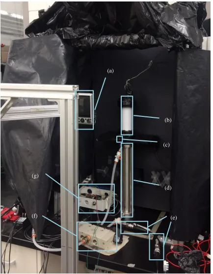
Figure 2-1 Overview of major components in the experimental apparatus: (a) high speed camera, (b) solid

vessel, (c) Red LED, (d) Pneumatic Actuator, (e) Pressure Transducers, (f) Double solenoid Valve, (g) Control

board with relays.

(d) (a)

(b)

(f) (g)

(c)

(27)

9 | P a g e

2.1 The vessel and others

A vessel made of Plexiglas, see figure 2-2 below, which is 26.5 cm long, 15.4 cm wide and 1.0 cm thick, is mounted on the piston plate through bolts and nuts. As for the dimensions the inner space has a diameter of 3.81 cm (or 1.5 inch), a wall thickness of 0.635 cm (or 0.25 inches), and a spool length (length of the inner volume) of 13.5 cm; The vessel is transparent and flanged for containing the phosphorescent particles. The transparent wall enabled image capture during mixing, which depicts how the solid bed was lifted, expanded and collapsed. Whereas, the overall length of the vessel including both flanges and bolts is 15.0 cm. This gives a total inner volume of 154 ml. Also note that as shown in figure 2-2, all surfaces were covered in black; for instance, the vessel wall at the back of the vessel is taped in black to make strong contrast with the white silica sand. The sand has a density of 2.65 g/cm3 with a Sauter-mean diameter close to 190 μm. Moreover, some of the frontal surface of the two vessel flanges facing the camera are covered in paper painted with non-reflective black dye.

The aluminum alloy plate acts as a support to the vessels and other units. This thickness of the platform plate further ensured the stiffness of the plate during rapid piston strokes while keeping all units on the plate at the same level.

(28)

10 | P a g e

Figure 2-2 Transparent JBR vessel; note that its backside (along with the platform) is covered in black tape

to make contrast with the white sand during JBR trials with the red LED wrapped in black showing only its

tip (see the boxed region).

(29)

11 | P a g e

2.2 Piston and valve complex

The piston used in this study is manufactured by BIMBA with model number FT-3112. It is a double acting FLAT-II model as depicted in part (d) of figure 2-1. For this piston is using dual rods connecting to a single rod end block, non-rotation operation is achieved. Hence, no alignment device such as guides or rods is required.

The body of the piston is built with 304-stainless steel. Anodized aluminum alloy makes up the piston heads. Piston rods are made of ground and polished 303-stainless steel. The sealing for the piston rods are Buna N O-rings while the rod bushing has oil impregnated bronze. The piston is capable to operate under a maximum air pressure rating of 200 psig within a temperature range of -25 °C to + 65 °C.

As for its physical dimensions, the piston cylinder bore size is 5.08 cm or (2 inches) with a stroke length of 30.48 cm (or 12 inches). The two air ports, at the top and bottom are designed to

accommodate 0.635 cm (or 1/4 inch) NPT fittings with an internal opening of 0.158 cm (or 1/16 inches). The mechanical drawings with exact dimensions provided by the manufacturer can be found in Appendix D.

2.3 Controller

The controller, shown in part (g) of figure 2-1, consists of two parts: Arduino UNO board and Sainsmart time relay. The Arduino board forms the backbone to implement the control algorithm. The detailed code of the Arduino control program can be found in Appendix C.

(30)

12 | P a g e

Figure 2-4 Arduino based feedforward relay controller (from:

https://reactivesystems.wordpress.com/2012/02/11/pneumatic-actuators/ ).

2.4 Valve and gas line

Compressed air is used in this thesis to actuate the piston. The air pressure is first set via adjusting the Metal work diaphragm regulator as seen in figure 2-6. Prior to performing any experiment, a global valve was connected directly downstream to the pressure regulator to act as an emergency shut-off valve. Further down the line is the 5-way 2-position bistable double solenoid valve (made by METALWORK with model #703001200U). The 2 positions are

(31)

13 | P a g e

Figure 2-5 METALWORK diaphragm air pressure regulator used for maintaining feed to the system.

Figure 2-6 Actual METALWORK 5/2 3/8 inch bistable double solenoid valve. Outlet

Exhaust

(32)

14 | P a g e

Pa

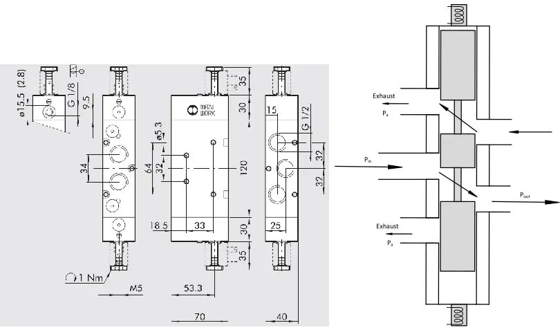
Figure 2-7 (a) Mechanical illustration of the METALWORK 5/2 3/8 inch bistable double solenoid valve along

with (b) its internal structure and the valve spool.

Initially, the solenoid valve switches direction, air passage on the right gradually increases, allowing air flowing to the lower chamber leading to upward motion of the piston. Once the designated time for maintaining the power signal is reached, solenoid valve switches direction. As a result, the air passage first decreases to zero and then increases for re-directing the air flow to the other piston chamber. The continuous alternation of the solenoid spool direction results in alternating directions of the piston motion.

2.5 Data Acquisition Devices (DAQ) and others

(33)

15 | P a g e

mechanical shaking that propagated to the working table. The camera stand has its location taped on the ground, as shown in figure 2-8. This allows researchers to check the camera’s position so that each recording can be kept as consistent as possible. In addition, prior to the start of each set of trials for a given repetition, the pixel to meter ratio is re-evaluated via performing a full stoke up and down test.

Figure 2-8 The bottom structure of the camera stand has its location taped on the ground.

Another important DAQ is the absolute pressure transducers. The transducers have an NPT head which is inserted between the lines connecting either piston nozzle to the solenoid valve ports. The maximum rating of the sensor is 100 psi in absolute pressure scale. They can be seen as part (e) of figure 2-1. The transducers are highly sensitive to the pressure change, with a response time of about 2 milliseconds. A complete surge voltage protection is also built in the sensor. The output of the transducer is also proportional to the pressure ranging from 0.5 to 5.0 Volts. The desired input for the transducer is 5.0 Volts. Before using these transducers, calibration is required, see section 4.1.1 for details. And the results can be seen in appendix D. Both

(34)

16 | P a g e

fluctuations and provide an additional surge protection. A closer look at the transducer sensor can be seen in figure 2-9.

Figure 2-9 Pressure transducer used in this study.

(35)

17 | P a g e

Figure 2-10 Black curtains setup around the workspace for light blocking: (a) is where the JBR was located;

(b) is position of the camera stand.

a

(36)

18 | P a g e

3 Piston motion modelling

3.1 Overview on piston operating principles

Overall, the solids within the vessel are carried upward and downward by the piston motion; thanks to inertia. To ensure effective and consistent mixing performance, the piston is required to have fast, accurate and periodic response. Low mechanical impedance and friction are also preferred. There are 3 types of actuators available for use: electrical, hydraulic and pneumatic. While electrical actuators may be accurate, they tend to be built with more sophistication and come at a very high cost. Hydraulic actuators are generally more complex to operate and

maintain. Pneumatic actuators are relatively inexpensive and are more responsive than hydraulic actuators. Since a constant supply of 100 psig dry and clean air is available in our laboratory, double acting pneumatic actuators become a good choice in our case.

Even though the working principles for pneumatic actuators sound quite easy to comprehend at a first glance, the actual model and control of this double acting piston can face numerous

challenges [Richer et al., 1999]. The first challenge is the highly non-linear air flow through the pneumatic components. Other issues include the distance between the compressed air source and pneumatic system, and potential thermodynamic and fluid dynamic changes during the piston operations. These factors complicate the flow calculations of the air through the system, especially when piston frequency increases [Gulati et al., 2005].

For this study, the overall JBR operations during a piston up stroke can be simply illustrated in the above figure 3-1. Here, the piston is initially at bottom prior to the experiments. Once the trial starts, air enters the lower piston chamber through lines and valves. The lower piston chamber expands as more air enters that chamber and drives the piston block upwards.

(37)

19 | P a g e Ball Valve

Air Pressure Regulator

Building Air Compressor

Piston Moves Up +

+

Air feed

Exhaust

Piston motion Air flow

Pa

Figure 3-1 Overall illustration of the air flow involved in piston modelling during upward stroke.

Ball Valve Air Pressure Regulator

Building Air Compressor

Piston Moves Up +

+

Air feed

Exhaust

Piston motion Air flow

Pa

(38)

20 | P a g e

Similarly, figure 3-2 shows that when air flow is reversed: air entering the upper piston chamber pushes the piston block downwards, forcing air out of the valve connected to the lower piston chamber. Alternating the air feed at the two ports under a given time difference thus leads to alternating piston up and down motion.

The piston model in this project considers the following terms: friction forces around the piston seals (coulomb and viscous friction forces), pressure drop across the double solenoid valve, piston gas port nozzle/orifice pressure drop, inactive volumes at either end of the strokes, tube pressure drop, and possible leakage between the upper and lower chambers.

3.2 Part I – Pressure feed adjustment

When calculating the mass flow of air that either enters or exits the piston chamber, one important assumption was made: all air flow upstream of the double solenoid valve is completely static with negligible flow rate. This assumption, according to literatures [Richer et al, 1999 & Mare et al, 2000], is reasonable when air source is a cylinder nearby. However, this is not the case here, as seen in figure 3-1 & 3-2. Prior to entering the solenoid valve, the air flow passes through a very long tube, and air flow is controlled by the ball valve and the air pressure regulator. As a result, the flow is not zero immediately upstream neither of the double solenoid valve nor between the valve and the piston when air exits a piston chamber. These relatively significant tube segments have to be taken into considerations since it is not valid to use compressible flow through orifice model to compute the mass flow of air (see section 3.3.2) without significant compromises on accuracies. To account these tube segments which air has to fill up prior to reaching the piston, a model called “virtual tube” is implemented.

The term virtual tube is denoted as Lv. This terms accounts for the entire tube segment upstream of the valve. Initially, air flow has to fill up all the lines and spaces upstream to the double solenoid valve. Besides, air needs to fill up the initial gap within the piston chamber. Overall, to take consideration of all the terms subject to air filling at the beginning of a trial, the equation becomes the following:

z

_0Total

= z

₀

+

At(Lt+Lv)

(39)

21 | P a g e

Here z0 is the initial gap between the piston’s moving block and its bottom plate. At is the cross sectional area of the tube. Lt is the tube connecting a double solenoid valve exit to a piston chamber. The piston chamber would have an effective cross sectional area with diameter of D. Lv is the virtual tube with the same cross sectional area as Lt; it is used to represent the space and lines upstream of the double solenoid valve. As part of the empirical parameter, Lv will be solved during the model fitting.

Overall, the required computation for part I can be summarized using the table 3-1:

Table 3-1 Input and output involved in virtual tube calculations.

Computation Model Conditions / Assumptions Input/ Given conditions Output

Virtual tube length, Lv

Flow is stagnant before entering the double solenoid valve (essentially a given orifice) after

taking account the length of the tube between air source and the

valve feed port Ideal gas law

Z0, initial gap between piston’s

moving block and the bottom plate

At, the cross sectional area of the tube Lt, the length of the tube

Z0Total, total initial length

of the tube

3.3 Part II – Air flow through the double solenoid valve

3.3.1 Overview

After adjusting the feed pressure to the double solenoid valve, the focus is then on how the internal structure, especially the displacement of the valve spool, affects the mass flow rate of the air. The key is to calculate the compressible air flow through a changing orifice within the

(40)

22 | P a g e

-Pa

Piston Moves Up +

+

PUv , GUv , At

PLv , GLv , At AUe

ALe

-Pa

Piston Moves Up +

+

PUv , GUv , At

PLv , GLv , At AUe

ALe

Fcontrol

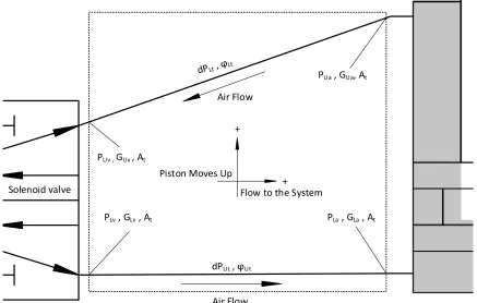
Figure 3-3 Part II detailed illustration for the valve and terms related when air flows through the valve filling

the lower piston chamber (left) and filling the upper piston chamber (right).

3.3.2 Calculating the compressible air flow through a given orifice

One of the major challenges in this study involve in air flow computation for the pneumatic system. Air flow is compressible. This makes it especially complex to calculate the pressure and mass flow rate of air when it is passing through a given orifice. In this study, air flow will encounter two changing orifices when it is passing through the valve. One of them is the orifice within the valve which has a changing diameter depending on the location of the spool. This orifice is relatively short, less than 8 mm; the other is at the piston nozzle, which has a fixed diameter, only about 3 ~ 5 mm, and a very small length, less than 5 mm.

(41)

23 | P a g e

speed. As a result, the kinetic energy dominates the total energy for air flow, and the change in potential energy can be treated as negligible. Therefore, the energy balance of the air flow through a given orifice can be explained using the following simplified equation:

h

_u

+

uu2

2

= h

d

+

ud2

2

= h

initial (3-2)

In the above energy balance, the subscript “u” and “d” represent the upstream and downstream side of the given orifice as the air flow is passing through. Whereas, “h” represents the enthalpy per unit mass of the air flow carries with it, or simply the specific enthalpy; “u” is the velocity of the air flow; i0 in this case would be the total initial specific enthalpy when the flow velocity is zero, or simply put it as the so-called “stagnation enthalpy” [Hougen et al., 1963]. As a result, the complete expression for the one-dimensional flow velocity becomes:

u = √2(h

₀

− h) = √2C

p

(T

0

− T) = √

2γRT_γ−10

(1 −

_TT

0

) (3-3)

Similar to the stagnation enthalpy, in equation 3-3, γ is the heat capacity ratio of air, which is constant in this study under the ambient lab conditions. This ratio is calculated using the

following simple equation: γ = C_Cp

v where Cp is the heat capacity of air under constant pressure,

and Cv is the heat capacity of air under constant volume. Both terms can be obtained from chemical engineering handbooks [Perry et al., 2007]. T0 is named as the stagnant temperature or temperature of the flow when it has a flow velocity of zero. Once again, the reasons for having these terms are to account for different flow situations: for instance, when air is flow out of the piston nozzle due to a short segment with very high flow velocity, the situation can be assumed

to be one dimensional and have equal-entropy. Therefore,_TT

0= (

P P0)

γ−1

γ _{, along with the formula of}

ideal gas law, P

ρ= RT, can be both used to substitute the relevant terms in equation (3-3), the resultant equation for calculating the air flow velocity becomes:

u = √2γ

γ−1

P

0

ρ

0

[1 − (

P P0

)

γ−1 γ

(42)

24 | P a g e

In this particular case of flow through a given orifice since the virtual tube has been used to correct the upstream pressure, and the upstream flow can be assumed to have zero velocity. For Td

Tu = (

Pd

Pu) γ−1

γ _{, derived from the formula of ideal gas law,}Pu

ρu = RTu , through a quick change in

subscripts, the following modified equations can be obtained:

u = √

_γ−12γ

P

_u

ρ

_u

[1 − (

Pd

Pu

)

γ−1

γ

(3-4b)

According to the continuity equation for mass flow of air, G = ρuA , based on the assumption of equal entropy and equation (3-4b) obtained earlier, the one-dimensional mass flow calculations under the equal-entropy condition can be expressed as:

G = A

_e

√

2γ

γ−1

P

u

ρ

u

[(

Pd

Pu

)

2

γ

_{− (}

Pd

Pu

)

γ+1

γ

_{] (3-5)}

From the above expressions, the mass flow is a function of the ratio between the upstream and downstream pressure across the orifice where air flow passes. This flow rate is also directly proportional to the effective cross sectional area of the passage.

Nevertheless, the actual mass flow calculations require further examination of the flow velocity. According to Ben-Dov and Salcudean [Ben-Dov et al., 1995], the flow calculations for velocity falling in the sonic and subsonic regime have their physical flow patterns differed significantly. To make a sound determination, the term critical pressure ratio, Ω, must be first obtained. Once this critical ratio is attained, constants for flow in subsonic or sonic regimes, C1 and C2 are calculated. These terms are independent of the operations and are generally related to the properties of the fluid using the following sets of equations:

C

₁

= √

_Rγ

(

_γ+12

)

γ+1 γ−1

(43)

25 | P a g e

C

₂

= √

_R(γ−1)2γ (3-6b)

Ω = (

_γ+12

)

γ−1γ

_(3-6c)

For air in this case, γ = 1.4, C1 = 0.040418, C2 = 0.156174 and Ω= 0.528. The above equation, although often used for ideal circular nozzle, is commonly used for all kinds of circular or elliptical valve orifices [Mare et al, 2000];

Note that here, the upstream, terms denoted with u, is always for the source of the air flow, downstream, terms denoted with d, is always where air flows. And during the formula

derivations, the upstream is always assumed to be stagnant, and thus having negligible kinetic energy with flow velocity set to be zero. Since the lab is air-conditioned, the temperature, T is constant throughout the study. The completed mass flow formula for air passing a specified nozzle is then established as the following:

if

Pd

Pu

≤ Ω,

dm

dt

= C

f

A

e

C

1 Pu

√T (3-7a)

if

Pd

Pu

> Ω,

dm

dt

= C

f

A

e

C

2 Pu

√T

(

Pd

Pu

)

1

γ

√1 − (

Pd

Pu

)

γ−1

γ _(3-7b)

(44)

26 | P a g e

Figure 3-4 Change of mass flow when flow is leaving an orifice (under same back pressure with changing

(45)

27 | P a g e

Figure 3-5 Change of mass flow when entering an orifice (under changing back pressure but with constant

upstream pressure).

3.3.3 5/2 double solenoid valve model

(46)

28 | P a g e

frequency. Consequently, the effects of valve delay cannot be simply neglected. This inspired a need to establish a valve model for calculating the real time effective area change for the air entering or leaving the valve. Nevertheless, the spool movement and its impact on regulating the air flow through the valve has to be understood.

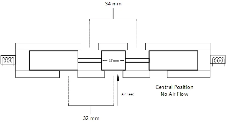
Before modelling the spool, it is necessary to first determine the size and the internal structure of the valve and the spool. Via taking the valve apart, some of the key dimensions are measured: the central block of the spool is about 17mm long; each of the two stems connecting the central block to the two side blocks of the spool is 17mm long each as well. Each port on the valve is half inch or 12.7 mm in diameter. The pitch for the two ports facing piston is 34 mm from center to center; and the pitch for the two ports on either side of the central air feed port is about 32 mm.

Figure 3-6 to 3-8 provide a concise presentation of the valve spool with respect to its location within the valve compartment as well as a brief illustration on how its location change affects the air passage. Note that the valve involved in this study is a 5-port 2-way double solenoid bistable valve, meaning it is symmetrically designed and operated without a neutral position at center. In figure 3-6, when the valve spool moves to its central location within the valve compartment, air feed is blocked completely. Neither air passage on either side of the valve is available.

(47)

29 | P a g e

Figure 3-7 When valve spool is at left position.

In figure 3-7, as the valve spool moves to its left most position, the left passage is open,

connecting the piston chamber and the atmosphere. Meanwhile, air enters the valve through the feed port and continues its flow towards the piston on the right port.

Figure 3-8 When valve spool is at right positon.

Figure 3-8 shows the exact opposite situation of figure 3-7. In this case, the right passage connecting the piston chamber and the atmosphere is open. Air feed enters the system through the left port. Since the magnetic force is applied to the spool during operations, the force balance for the spool can be developed as the following expression:

(48)

30 | P a g e

In this equation, Ms stands for the mass of the valve spool; Ffs stands for an overall term for sum of the Coulomb and kinetic friction during valve operations. In addition, x stands for the

(horizontal) displacement of the spool within the valve. d 2_x

dt2 stands for the acceleration of the spool. Fc is the net controlling force acting on the spool. In order not to damage the integrity of the valve structure, the internal structure was not measured. Therefore, the mass of the spool is unavailable. Through the limited external measurement of the hardware, it was found that the maximum displacement of the spool from left to right is 17 mm. If the spool’s left most location is defined as x=0, the direction towards right is positive. The given mechanical delay of 30 milliseconds can be viewed as the time it takes for the valve spool to travel from one side to another.

Also note that according to the manufacturer, this valve is designed to have minimum maintenance and friction. To preserve the outstanding performance of the valve, sufficient lubrication has been applied regularly to minimize the friction and flush out deposits left in the internal structure during each trial. The overall time and distance for the spool to travel is relatively short. This means that the force applied by the solenoids onto the spool, Fc is much larger than the friction forces Ffs. To simplify the expression, Ffs is assumed to be zero in this study for the spool. As a first order approximation, the acceleration for the spool when it is moving along the internal structure of the valve is taken as a constant. Since the denominator, Ms is also a constant, the overall quotient is denoted as a constant as, which represents the

acceleration of the spool. Therefore, equation (3-8a) can be simplified as the following:

M

_sd2x

dt2

≅ F

c (3-8b)

Subsequently, a system of differential equations with the above boundary conditions is established as the following:

when 0 < t < 0.03, d

2_x

dt2 =

Fc

Ms≅ as, else

d2x

dt2 = 0 (3-9a)

dx

dt = ∫

d2_x

dt2

t

0 dt, when t = 0,

dx

dt = 0; when t = 0.03,

dx

(49)

31 | P a g e

x = ∫₀tdx_dtdt, when t=0, x = 0; when t = 0.03s, x = 0.017m (3-9c)

The analytical solution for the above system then becomes the following:

x = as

2 t2+ Constant1∗ t + Constant2

Whereas, “Constant1” and “Constant2” in the above equation are both arbitrary constants generated from the analytical integrations. After applying the given boundary conditions, the kinetic expressions for the valve spool displacement can be simplified as:

x =

37.78

2

𝑡

2_(3-10)

The above equation calculates the displacement of the spool at a given time; however, this is not sufficient, as the spool moves, the effective opening area for air pass through the valve changes. Fortunately, the effective cross sectional area can be integrated with a given range of spool displacement within the valve. The following sketch, figure 3-9, taken from [Richer et al., 1999], serves as an illustration of the pertinent relationship.

Figure 3-9 Illustrates the relationship between the valve spool and valve opening [Richer et al., 1999].

(50)

32 | P a g e

exits from the other side, its area changes as the spool’s location changes. In case the side where air enters has a cross sectional area different from the side air exits or vice versa, the smaller area of the two will be selected as the effective opening for air flow calculations. In general, the effective cross sectional area is computed using the following formula:

Ae = 2 ∫ √R₀xe h2− (ξ − Rh)2dξ (3-11)

After conducting implicit integration, the resultant formula becomes:

A_e = 2R_h2cot (√ xe

2Rh−xe) − (Rh− xe)√xe(2Rh− xe) (3-12)

However, the spool moves back and forth over time which implies that this effective area is in a rather periodic relationship with the spool’s displacement. Subsequently, the area needs to be calculated over different boundaries. Nevertheless, whenever the calculated Ae is larger than the cross sectional area of the tube, At, the former will be over-written by the value of At since the cross sectional area of the tube connected to the valve is the maximum cap of the effective cross sectional area of the flow through a given orifice.

Using xeL as the term that describes the effective displacement of the spool that covers the left hand side valve port, connecting to the piston, and xeU as the term that describes the effective displacement of the spool that covers the right hand side valve port, assuming that the left part of the valve passage is connected to the lower piston chamber, and the upper piston chamber is connected to the right part, the resultant spool movement can be broken down into seven cases as shown in table 3-2.

(51)

33 | P a g e

Table 3-2 The seven cases of spool position and the resultant air passage situation within the valve.

Spool Displacement

(x, mm)

Air Flow at Left Passage

Condition

Air Flow at Right Passage

Condition

Effective Left Displacement

(xeL, mm)

Effective Right Displacement

(xeU, mm)

0<x<1 Outflow Inflow 6.35+x 6.35-x

1<x<6.35 Outflow Inflow 8.35-x 6.35-x

6.35<x<8.35 Outflow Close 8.35-x 0

8.35<x<8.65 Close Close 0 0

8.65<x<10.65 Close Outflow 0 x-8.65

10.65<x<16 Inflow Outflow x-10.65 x-8.65

16<x<17 Inflow Outflow x-10.65 3*6.35+4.3-x

Taking the left most location of the spool as zero ensures positive displacement readings for the spool throughout this study. Recall the previously presented equations in (3-6) for computing mass flow of a compressible flow through a given orifice shown in section 3.3.2. To find the mass flow of air through the valve, it can be calculated using the obtained Ae and applying the equations in the previous section to this valve condition:

The upstream pressure Pu becomes Pin, the air pressure fed to the valve; and the downstream pressure becomes PLv or PUv depending on which piston chamber air flow is directed to. Similarly, the mass flow rate becomes either GLv or GUv. For instance, as illustrated in the left part of figure 3-4, assuming that air enters the valve and flows to the lower chamber, the overall mass flow rate, GLV, leaving the valve can be expressed using the following equations:

if

PLv

≤ Ω, G

Lv

= C

f

A

e

C

1

(52)

34 | P a g e

if

PLv

> Ω, G

Lv

= C

f

A

e

C

2

√T

(

PLv

)

1

γ

√1 − (

PLv

)

γ−1

γ _(3-13b)

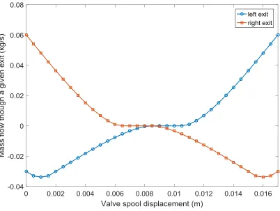
To better visualize the relationship between the change of effective valve orifice area and the mass flow of air exiting the valve, figure 3-10 is attached. Note that the positive mass flow rate indicates air entering a piston chamber through the valve. Whereas, the negative mass flow rate indicates air leaving a piston chamber before entering the valve. The latter is estimated via setting the exhaust pressure as atmospheric pressure and back calculates the pressure before air flow entering the valve. Table 3-3 is provided to give a recap on what has been covered in this part of the model.

Figure 3-10 Mass flow through the valve as a function of spool displacement.

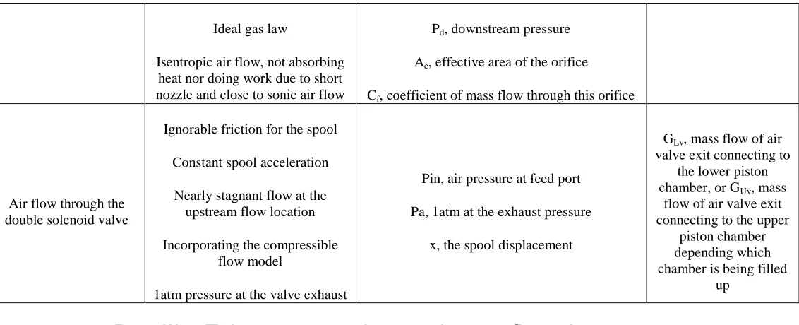
Table 3-3 Input and output summary for the double solenoid valve model.

Required calculations Assumptions / Conditions Input Output

Compressible flow

through a given orifice Ideal nozzle Pu, upstream pressure

dm

(53)

35 | P a g e

Ideal gas law

Isentropic air flow, not absorbing heat nor doing work due to short nozzle and close to sonic air flow

Pd, downstream pressure Ae, effective area of the orifice Cf, coefficient of mass flow through this orifice

Air flow through the double solenoid valve

Ignorable friction for the spool Constant spool acceleration Nearly stagnant flow at the

upstream flow location Incorporating the compressible

flow model

1atm pressure at the valve exhaust

Pin, air pressure at feed port Pa, 1atm at the exhaust pressure

x, the spool displacement

GLv, mass flow of air valve exit connecting to

the lower piston chamber, or GUv, mass

flow of air valve exit connecting to the upper

piston chamber depending which chamber is being filled

up

3.4 Part III – Tube pressure drop and mass flow changes

3.4.1 Overview

(54)

36 | P a g e

Solenoid valve

PUv , GUv , At

PLv , GLv , At

PUa , GUa, At

PLa , GLa , At

dPUt , ϕUt

Piston Moves Up +

+

Figure 3-11 Part III boundaries and related terms (enclosed by the dashed box).

3.4.2 Tube pressure drop model

Previously, many argued that the air flow will become laminar along the tube; some increase the step numbers for solving the equations, some use second order linear approximation to estimate this propagation of the air flow [Schuder et al., 1959 & Anderson et al., 1967 & Hougen et al., 1963]. However, the primary focus of this study is on the piston motion. It is not necessary to bring up the complex correlations for obtaining the pressure drop and flow reduction over a relatively short 3/8 inch tube segment. Meanwhile, flow rate in the study often gets close to or even exceeds the laminar turbulent boundary.

For sake of having a simple yet robust approximation, instead of solving the complex continuous system of equations analytically, a numerical method involving in discretizing the tube segment into dozens of sub-sections are applied to solve this problem. In this case, the tube is divided into a dozen of sub-sections with length s. Within each sub-section, the air density is assumed

(55)

37 | P a g e

direction of the flow through incrementally adding the distance and time as illustrated in figure 3-12, the notations are the following: P is the absolute pressure; dP is for the pressure drop; G is mass flow; φ is the reduction coefficient of mass flow of air; ρ is the density of air within a given sub-section.

1 2 3 4 5 6 7 8 n-1 n

P(0,t0) , G(0,t0)

P(1,t1) , G(1,t1)

P(Ltube,tn) , G(Ltube,tn)

+ s

dP1 , ϕ1 , ρ1 dPn , ϕn , ρn

P(n-1,t(n-1)) , G(n-1,t(n-1))

Ltube

Dtu

b

e

Figure 3-12 Numerical approximation of pressure drop and flow reduction along the tube through

discretization.

Subsequently, the following partial differential equations are used to accomplish this task:

∂P

∂s

= −R

t

u − ρ

∂u

∂t (3-14)

∂u ∂s

= −

1 ρc2

∂P

∂t (3-15)

In addition to the terms appeared in figure 3-13, u is the air flow velocity within the tube; c is the sonic speed at the ambient lab condition; s is the incremental segment of the tube; Rt is the resistance of the tube. If set At as the cross sectional area of the tube segment, the mass flow rate through a given tube segment simply becomes 𝐺_𝑡 = 𝑑𝑚_𝑑𝑡𝑡 = ρ𝐴_𝑡𝑢 Using the substitution

methods suggested by the literature [Elmadbouly et al., 1994], inserting the previous mass flow rate expressions into equation 14 and 15, the resultant formula for mass flow of air as time and location changes is the following:

∂2G_𝑡

∂t2

− 𝑐

2 ∂ 2_G

𝑡

∂s2

+

R_𝑡 ρ

∂G_𝑡

(56)

38 | P a g e

The above equation is in fact a wave function with a dissipative term. Introducing the term,

G_t(s, t) = φ(t)v(s, t) and substitute it for the term Gt in the above equation, and solve it

according to [Chester et al., 1970]. When the term φ(t) = e−(

Rt

2ρ)t_{is defined, the resultant}

solution for v(s, t) is a discrete hyperbolic function.

Since the tube is relatively short, less than 0.5 meters long, the scattering can be ignored and the equation becomes essentially a classical wave equation. Moreover, assume at t=0, there is no flow; the flow near the starting point of the tube, s=0, can be denoted as the term q (t). All these terms can be seen in figure 3-13 for a simplified illustration. Also, assume there is no reflection nor back flow taking place in the tube, using the term Lt to represent the length of the tube, the overall initial condition becomes the following:

{

v(s, 0) = 0

∂v

∂t(s, 0) = 0

v(0, t) = q(t)

(3-17)

P(0,t0) , G(0,t0) = q(t0) P(Lt,tn) , G(Lt,tn)

+ s

Lt

At

Figure 3-13 Illustration of the flow entering and leaving a tube.

Since air propagates as a sound wave travelling within the tube, the flow will reach the exit after a certain time τ = Lt/c. Solving v(s, t) for φ (t) gives the following:

v(s, t) = {0 , if (t <

s c)

q (t −s_c) , if (t >s_c) (3-18)

(57)

39 | P a g e

For a 50 cm long tube, the physical time delay as a result of sonic wave propagation is about 1.5 milliseconds. This delay is relatively insignificant, only 5% of the valve response time, 30 milliseconds. Therefore, this time delay is ignored in this study. While the piston operates continuously within the given run time, the corrected formula for computing the mass flow rate becomes:

G_t(L_t, t) = e−(RtRT2P )(Ltc)h(t)

_(3-20)

Note that the P in the above expression represents the air pressure near the exit end of the tube segment. Overall, this function relates the exit mass flow of the air to the inlet mass flow of the air. According to [Hougen et al., 1963], this function performs reasonably well over a short tube segment with lower air feed frequency. As for the term Rt, it can be attained via calculating the pressure drop along the tube using Darcy–Weisbach equation with Fanning friction factor [Munson et al., 1990] (note that the specific weight of air is multiplied at both sides of the original equation):

ΔP = fLt

D ρu2

2 = RtuLt (3-21)

In the above equation, f is the Fanning friction factor; D is the tube diameter. For fully developed laminar flow, f = 64/Re where Re is the Reynolds number. Subsequently, for laminar flow the tube resistance becomes [Schuder et al., 1959]:

R_t =32μ_D₂ (3-22)

In the above equation, μ is the kinetic viscosity of air. For turbulent flow passing through, the inner wall of the 3/8 inch soft plastic tube is assumed to be smooth; thus, the friction factor can be calculated as f = _Re0.316_0.25 , according to Poiseuille's law. After substituting into equation (3-21) using the Blasius equation, the tube resistance formula can be simplified as the following [Jukka et al., 2011]:

(58)

40 | P a g e

This Rt is then substituted back in equation (3-21) to calculate the mass flow of air at a given spot along the tube at a given time. Also note that when calculating along the direction of the flow, pressures drop ΔP is negative, the reduction of mass flow φ at a given time is less than 1. Using the terms labelled in figure 3-13, Pout and Gout are calculated with given Pin, and initial flow and tube properties in this case.

However, when computing the tube with air flows out of the piston towards valve in the same time, the way to calculate these terms are slightly different. In this case, Pout and Gout are given (as estimated using the pressure drop obtained from the valve model via setting the exhaust pressure close to 1 atmosphere, see details in section 1.3.3). The pressure drop and flow changes are added incrementally and backwardly since the calculation starts near the valve, which is the end point of air flow in the tube. The model then progressively back calculates the pressure and flow rate one sub- section upstream of current point till it reaches the point when air first enters the tube from the piston nozzle.

3.4.3 Selecting the number of steps

(59)

41 | P a g e

Figure 3-14 Percent errors in pressure drop calculations vs. number of steps.

(60)

42 | P a g e

Figure 3-15 Percent errors in mass flow calculations with number of steps.

To summarize, equation (3-20) and (3-23) are both used for taking the flow reduction along the tube into considerations using the Blasius formula. Prior to calculations, mass flow is used to find the Reynolds number. Although this model avoided solving the complex partial differential equations in (3-16), obtaining the changing pressure and flow rate of the compressible air flow along the tube require numerical integration whose accuracy depends on the number of steps. A summary is provided in table 3-4 below.

Table 3-4 Input and output summary for tube delay model.

Required calculations Conditions / Assumptions Input Output

Pressure drop and flow reduction along the tube (always compute from the valve side to piston side)

Sonic speed over the relatively short tubes caused no delay of air flow in time No flow at the starting point of the tube at

beginning

GUv or GLv, mass flow of air entering the tube, depending on the direction

of the flow PUv or PLv, pressure of air

GUa or GLa, mass flow of air leaving the tube,

Piston Modelling and Gas-Solid Mixing Characterization in JBR

Scholarship@Western

Scholarship@Western

Piston Modelling and Gas-Solid Mixing Characterization in JBR

Piston Modelling and Gas-Solid Mixing Characterization in JBR

Keywords

Co-Authorship Statement (where applicable)

Acknowledgments

Table of Contents

List of Tables

List of Figures

LIST OF ABBREVIATIONS / NOMENCLATURE

1

Introduction

1.1

Motivations to further develop the JBR system

1.2

Assessing solid mixing

1.3

Objectives and scope

2

Experimental Setup

2.1

The vessel and others

2.2

Piston and valve complex

2.3

Controller

2.4

Valve and gas line

2.5

Data Acquisition Devices (DAQ) and others

3

Piston motion modelling

3.1

Overview on piston operating principles

3.2

Part I – Pressure feed adjustment

z

= z

+

3.3

Part II – Air flow through the double solenoid valve

3.3.1

Overview

3.3.2

Calculating the compressible air flow through a given orifice

h

+

= h

+

= h

u = √2(h

− h) = √2C

(T

− T) = √

(1 −

) (3-3)

P

ρ

[1 − (

)

u = √

P

ρ

[1 − (

)

G = A

√

P

ρ

[(

)

− (

)

] (3-5)

C

= √

(

)

_{− (}

_{] (3-5)}