www.ijiset.com
Determination of Component Values for Butterworth Type Active Filter
by Differential Evolution Algorithm
Bahadır Hiçdurmaz
Department of Electrical & Electronics Engineering, Dumlupınar University, Kütahya, 43100, Turkey
Abstract
In the implementation of active filters, it is cost-effective to determine the passive component values from a range of manufactured preferred values. In conventionally design method, component values results in values that do not all comply with preferred values and the designer chooses the nearest preferred value thence causing a design deviation. So, in order to reduce this problem, various metaheuristic algorithms are used in literature. In this paper, the applicable of differential evolution (DE) algorithm for 10th-order Butterworth active filter is investigated. It is seen that DE algorithm gives quite good results in order to get ideal filter parameters. Furthermore, according to obtained results, DE algorithm gives better design results than backtracking search algorithm (BSA) which is used in another similar study.
Keywords: Active Low-Pass Filter, Differential Evolution
Algorithm, 10th-order Butterworth Type, Sallen-Key Topology.
1. Introduction
Electronic filters are frequency-selective circuit elements that pass electrical signals in specified frequency ranges without any change and stop electrical signals in other frequencies [1], [2]. Filters find use in a variety of electrical and electronic applications such as audio signaling, instruments, sound and signal sources, television and radio broadcasts and data communications. For example, they are utilized to acquire dc voltages in power supplies, cut off noise in communication channels, split radio and television channels from the multiplexed signal provided by antennas.
When designing a filter circuit, the values of the selected circuit elements are calculated according to the determined design conditions and the used equations. In order to reduce the calculation process, the values of some discrete elements used in circuit design are chosen equal to each other. However, in this conventional method, there is a problem that the values of the other discrete elements to be used do not exactly match the standart serial values. Then, the performance of the designed circuit can be reduced by depending on the values of the elements selected closest to the designed values. Thus, the characteristic of the designed circuit deviates from the ideal characteristic and
the error rate increases. In recent years, heuristic algorithms derived from artificial intelligence and natural science have begun to be used instead of traditional methods in finding optimal values of filters designed with discrete elements. The popular ones of these algorithms are differential evolution (DE), particle swarm optimization (PSO), genetic algorithm (GA), artificial bee colony (ABC), tabu search (TS) and backtracking search algorithm (BSA). The component values obtained by these algorithms can be rounded to the nearest standard component values and fewer design errors can be achieved
than with the conventional method. In [3], 3rd and 4th-order
Butterworth and Chebyshev low pass filters (LPFs) were designed using ABC and PSO. The results show that the transfer characteristic obtained by ABC has the sharpest descent in transition band while PSO is much approximated to ideal characteristic in passband. Another study of filter design is given in [4]. In here, Simplex-PSO
algorithm was used for designing of 4th - order Butterworth
active LPF and 2nd-order State Variable active LPF.
According to obtained results, Simplex-PSO algorithm exhibited less total design error than the reported methods.
Furthermore, 10th-order Butterworth LPF and 10th-order
Butterworth high-pass filter (HPF) were designed by using BSA in [5] and [6], respectively. Other related works in this topic are given in [7], [8], [9], [10], [11], [12], [13].
In this work, a 10th-order Butterworth LPF in Sallen-Key
Topology is designed by DE utilized for selection of filter
circuit’s component values. FSF and Q values of designed
circuit are calculated according to optimized component values. These results are compared with both ideal
Butterworth FSF and Q values and the results obtained by
BSA.
2. Sallen-Key Topology Butterworth LPF
An active LPF, which is one of the main active filters, is an electronic device that allows all frequency components below its cut-off frequency and rejects or attenuates all
frequency components above. In Fig. 1, a 2nd-order
www.ijiset.com
Fig. 1 2nd-order unity-gain Sallen Key LPF architecture
From circuit analysis, transfer function, is obtained
as
(1)
In equation (1), substituting gives
(2)
The standard form of is expressed as [15]
(3)
where is the cut-off frequency,
is frequency scaling factor,
and is the quality
factor.
Then, the amplitude response of the filter is found as
(4)
A 10th-order LPF are constructed by cascading five 2nd-
order stages. The ideal FSF and Q values of each stage for
10th-order Butterworth LPF are given in Table 1 [15]. In
this study, the filter circuit was designed for cut-off frequency of 10 kHz.
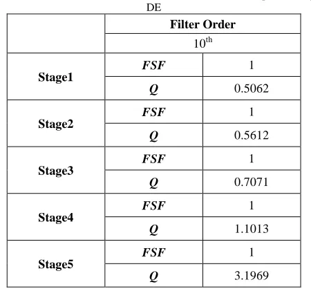
Table 1: FSF and Q values of ideal 10th-order Butterworth Filter
Filter Order
10th
Stage1 FSF 1
Q 0.5062
Stage2 FSF 1
Q 0.5612
Stage3 FSF 1
Q 0.7071
Stage4 FSF 1
Q 1.1013
Stage5 FSF 1
Q 3.1969
3. Differential Evolution (DE) Algorithm
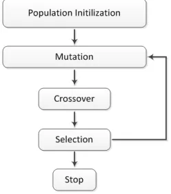
DE is a heuristic optimization technique based on genetic algorithm (GA) in operation [16], [17]. Although DE has the same operators with GA, its structure and implementation are different from those of GA. DE is a very simple but a very powerful population-based stochastic global optimizer. The flow chart of DE is shown in Fig. 2.
Fig. 2 The flow chart of DE algorithm
The parameters of DE are the population size NP, the
number of parameters D, the generation number g, the
crossover rate CR and the scaling factor F.
3.1 Population Initialization
In the application of DE, before the initialization of the population, both upper and lower bounds for each parameter are defined. Then, a random number generator assigns a value for each parameter of every vector a value from the prescribed range. The initial population created
by NPD-dimensional vectors can be described with
(5)
where is the jth parameter of the ith vector in the
generation g for j=1,2,…,NP ; g=0,1,…,gmax. and
are the lower and upper bounds of parameters, respectively.
randj[0,1] is a uniformly distributed random number for
the jth parameter in the range of [0,1].
3.2 Mutation
The mutation is to make random changes on the parameters of the vectors. After the initialization, DE
mutates and recombines the population of NP trial vectors.
At first, a base vector index r0, which is different from the
target vector index i, to be subjected to mutation, is
randomly chosen from the initial population. And also, the
www.ijiset.com
other and from both the base and target vector indices, are randomly selected once per mutant. Then, mutation process is started. In mutation process, the vectors
randomly chosen with vector indices r1 and r2 are
subtracted from each other and the difference is multiplied
by a specified F number. The obtained weighted
differential vector is added to the base vector
0
, ,
j r g
x to
produce a mutant vector vj i g, , . The mutant vector can be
expressed with
(
)
, , , , , , , ,
: .
∀ ≤ = + −
o 1 2
j i g j r g j r g j r g
j D v x F x x (6)
where the scaling factor F, is a real number controlling the
rate at which the population evolves and it generally takes a value in the range of (0,1).
If the parameters of the generated vector exceed the minimum or maximum bound component values, they are changed according to (7).
( ) ( )
, ( ) ( )
,
,
<
= > l l
j j j
j i u u
j j j
x if x x
v
x if x x
(7)
3.3 Crossover
In the crossover process, the trial vector uj,i,g is created by
using the mutant vector vj,i,g and target vector xj,i,g. The
parameters of this new generated vector are chosen from
the mutant vector with a probability of CR. Otherwise,
parameters are copied from the target vector. Also, j=jrand
condition is used in order to guarantee the choice of at least one parameter from the mutant vector. The trial vector created as the result of crossover is given by
[ ]
, , , , , , : 0,1 ∀ ≤ ≤ ∪ = = j i g rand
j i g
j i g
j D
v if rand CR j j
u
x otherwise
(8)
The criterium used for determination of the vector that will be transferred to the next generation, i.e. the target vector or the trial vector, is the convenience. The convenience value of the target vector has already been known. However, the convenience value of the trial vector must be computed.
3.4 Selection and Termination of the Algorithm
The vector having the highest convenience value between the target and the trial vectors is assigned to the next generation. If the purpose of the optimization is minimization, the expression for the selection process can be given by
, , , , 1 , : , ( ) ( ) , + ∀ ≤ ≤ =
i g i i g i i g
i g
i g
i NP
u if f u f x
x
x otherwise
(9)
where f(x) is the objective function intended to be
optimized. This operation cycle continues until g=gmax.
When termination criterium is satisfied, the best current
vector is taken as the solution. gmax is the defined iteration
number to terminate the algorithm.
4. Simulation and Results
The aim of this study is to get ideal FSF and Q values for
10th–order Butterworth type active filter with optimized
component values by using DE algorithm. When applying DE to this optimization problem, each passive component of filter belonging to each stage was encoded in the string form as shown in Table 2. In this case, the components values of the filter are successively adjusted by DE until the error is minimized. The design error of the filter,
Total
Error is the summation of the cost function errors of
FSF and Q, Error1 and Error2respectively, given in [5].
5 , 1 1 , 5 , 2 1 ,
1 (1 ) 2
= = − = − = = × + − ×
∑
∑
t i i
i t i
t i i
i t i
Total FSF FSF Error FSF Q Q Error Q
Error α Error α Error
(10)
where FSFt i, is target FSF, Qt i, target quality factor, and
α is the constant (α=0.5). The aim is to keep the total
error as low as possible. So, ErrorTotal is the objective
function of the design problem.
Table 2: Representing the component values in the string form
Stage1 … Stage5
R11 C11 R21 C21 … R15 C15 R25 C25
The designed DE code for the filter was written in MATLAB R2015a and run in a computer with INTEL Core i7 2.4 GHz processor and 8 GB RAM memory.
In the simulation studies, the population size NP is 25 and
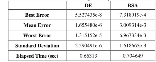
iteration number is set to 1000 for DE. Experiments are performed over 25 independent runs. Obtained results are presented in Table 3-5.
Table 3: Statistical results of design for independent 25 runs
DE BSA
Best Error 5.527435e-8 7.318919e-4
Mean Error 1.655480e-6 3.009314e-3
Worst Error 1.315152e-5 6.967334e-3
Standard Deviation 2.590491e-6 1.618665e-3
www.ijiset.com Table 4: FSF and Q values of 10th-order Butterworth Filter optimized by
DE
Filter Order
10th
Stage1
FSF 1
Q 0.5062
Stage2 FSF
1
Q 0.5612
Stage3
FSF 1
Q 0.7071
Stage4
FSF 1
Q 1.1013
Stage5
FSF 1
Q 3.1969
Table 5: Component values of best solution obtained by DE
Component Stage1 Stage2 Stage3 Stage4 Stage5
R1(kΩ) 1.87948 4.48693 2.63646 2.489 1.3411
R2(kΩ) 2.57258 2.43548 1.99927 3.35576 3.63435
C1(nF) 7.06215 4.0968 4.85535 2.47256 1.0006
C2(nF) 7.41817 5.65798 9.89751 12.2653 51.939
Furthermore, in Table 3, BSA design results of the same filter are obtained as a product of another study, given in [5]. It is apparent that DE gave better results than BSA. According to the results obtained by DE algorithm, it is possible to realize circuit designs very close to the ideal cases. Optimized component values are given in Table 5. These values can be rounded to the nearest standart component values and acceptable errors can be obtained. The gain curves of each stage obtained by DE and total gain curves for target and computed solutions are plotted in Fig. 3 and Fig. 4, respectively.
Frequency ( kHz )
10-1
100
101
102
Gains ( dB )
-50 -40 -30 -20 -10 0 10 20
Stage 1 Stage 2 Stage 3 Stage 4 Stage 5
Fig. 3 Gain curves of each filter stage obtained by DE
Frequency ( kHz )
10-1 100 101 102
Total Gain ( dB )
-50 -45 -40 -35 -30 -25 -20 -15 -10 -5 0 5
Target Computed
Fig. 4 Total gain curves for target and computed solutions
Fig. 5 shows the cost function versus iteration number. In this figure, it can be seen that DE designs an acceptable filter at around 200 iterations. This is the very fast convergence rate.
Iteration Number
0 100 200 300 400 500 600 700 800 900 1000
Cost Function
0 0.2 0.4 0.6 0.8 1 1.2
Fig. 5 The cost function versus iteration number
5. Conclusion
In this study, an application of DE algorithm has been achieved for the component selection of analog active filter
design. The 10th-order Butterworth low pass filter design
has been investigated for the prediction of component values. It is apparently seen that DE successfully minimized the design error in a short computation time. From the obtained results, DE algorithm is considered to be able to used efficiently for more complex circuit design in future works.
References
[1] D. Lancaster, "Active Filter Cookbook", Howard W. Sams & Co., 1975.
[2] S. A. Pactitis, "Active Filters Theory and Design", CRC Press, Taylor & Francis Group, 2007.
www.ijiset.com 2011 7th International Conference on Electrical and Electronics Engineering, 1-4 December, Bursa, TURKEY.
[4] B. P. De, R. Kar, D. Mandal, S. P. Ghoshal, "Optimal Selection of Components Value for Analog Active Filter Design Using Simplex Particle Swarm Optimization", Int. J. Mach. Learn. & Cyber., pp. 621-636, 2015. [5] B. Hiçdurmaz, B. Durmuş, H. Temurtaş, S. Özyön, "The
Prediction of Butterworth Type Active Filter Parameters in Low-Pass Sallen-Key Topology by Back Tracking Search Algorithm", 2nd International Conference on Engineering and Natural Sciences (ICENS 2016) , Chapter 9, pp.2422-2428, 24-28 May 2016, Sarajevo, Bosnia and Herzegovina. ISBN 978-605-83575-0-1. [6] B. Durmuş, B. Hiçdurmaz, H. Temurtaş, S. Özyön,
"Defining the Parameters of the High-Pass Active Filter by Using Backtracking Search Algorithm", 2nd International Conference on Engineering and Natural Sciences (ICENS 2016) , Chapter 9, pp.2429-2435, 24-28 May 2016, Sarajevo, Bosnia and Herzegovina. ISBN 978-605-83575-0-1.
[7] D. H. Horrocks, Y. M. A. Khalifa, "Genetically Derived Filters Circuits Using Preferred Value Components", In Proc. IEE Colloquium on Analogue Signal Processing, 1994, p. 4/1-4/5.
[8] A. Kalinli, "Component Value Selection for Active Filters Using Parallel Tabu Search Algorithm", Int, J. Electron. Commun., Vol. 60, pp. 85-92, Jan. 2006.
[9] A. F. Sheta, "Analogue Filter Design Using Differential Evolution", Int. J. Bio-Inspired Comput., Vol. 2 (3), pp. 233-241, 2010.
[10] C. Goh, Y. Li, "GA Automated Design and Synthesis of Analog Circuits with Practical Constraints", In Proc. CEC2001, 2001, Vol. 2, p. 170-177.
[11] R. A. Vural, T. Yıldırım, T. Kadioğlu, A. Basargan, "Performance Evaluation of Evolutionary Algorithms for Optimal Filter Design", IEEE Trans. Evolut. Comput., Vol. 16, pp. 135-147, Feb. 2012.
[12] R. A. Vural, T. Yıldırım. "Component Value Selection for Analog Active Filter Using Particle Swarm Optimization", In Proc. ICCAE, 2010, Vol. 1, p. 25-28.
[13] D. Ustun, M. Akkus, M. B. Bicer, H. Temurtas, A. Akdagli, "Sezgisel Algoritmalar ile Butterworth ve Chebyshev Alçak Geçiren Filtre Tasarımı", SIU-2015 Sinyal İşleme ve İletişim Uygulamaları Kurultayı, 16-19 Mayıs 2015, p. 108-111.
[14] R. P. Sallen, E. L. Key, "A Practical Method of Designing RC Active Filters", IRE Transactions-Circuit Theory, 1955.
[15] J. Karki, "Active Low-Pass Filter Design", Texas Instruments, Dallas-Texas, Application Rep. SLOA049B, 2002.
[16] K. V. Price, R. M. Storn and J. A. Lampinen, "Differential Evolution: A Practical Approach to Global Optimization", Springer-Verlag, Berlin Heidelberg, 2005.
[17] A. Qing, Differential Evolution: Fundamentals and Applications in Electrical Engineering, John Wiley &Sons (Asia) Pte Ltd., 2009.