Effective apsidal precession in oblate coordinates
Abra˜
ao J. S. Capistrano
1,2?, Paola T. Z. Seidel
1†
, Lu´ıs A. Cabral
1,3‡
1Applied physics graduation program, UNILA, 85867-670, P.o.b: 2123, Foz do Igua¸cu-PR, Brazil2Casimiro Montenegro Filho Astronomy Center, Itaipu Technological Park, 85867-900, Foz do Igua¸cu-PR, Brazil 3Universidade Federal do Tocantins, Curso de F´ısica, Setor Cimba, Aragua´ına - TO, 77824-838, Brazil
Accepted Received ; in original form
ABSTRACT
We use oblate coordinates to study its resulting orbit equations. Their related solutions of Einstein’s vacuum equations can be written as a linear combination of Legendre polynomials of positive definite integersl. Starting from solutions of the zeroth order
l = 0 in a nearly newtonian regime, we obtain a non-trivial formula favoring both retrograde and advanced solutions for the apsidal precession depending on parame-ters related to the metric coefficients, particularly applied to the apsidal precessions of Mercury and asteroids (Icarus and 2 Pallas). As a realization of the equivalence problem in general Relativity, a comparison is made with the resulting perihelion shift produced by Weyl cylindric coordinates and the Schwarzschild solution analyzing how different geometries of space-time influence on solutions in astrophysical phenomena.
Key words: perihelion, gravity
INTRODUCTION 1
Since the explanation of the perihelion advance of Mer-cury by Einstein in 1915 as application of general Relativity (GR), and it has been considered one of the fundamental laboratories for testing extensions of standard GR and other gravitational models such as, e.g, the modification of New-tonian Dynamics (MOND)(Schmidt 2008), Kaluza-Klein five-dimensional gravity (Lim and Wesson 1992), Yukawa-like Modified Gravity (Iorio 2008a), Horava-Lifshitz gravity (Harko, 2011), brane-world models and variants (Mak and Harko 2004; Maia, Capistrano and Muller 2009; Cheung and Xu 2013; Chakraborty and Sengupta 2014; Jalalzadeh et al. 2009; Iorio 2009a,b) and in the parametric post-Newtonian (PPN) framework and beyond and approaches in the weak field/slow motion limits (Avalos-Vargas and Ares de Parga 2012; Arakida 2013; Adkins and McDonnell 2007; Biswas and Mani 2005; D’Eliseo 2012; Deng and Xie 2014; Feldman 2013; Li et al. 2014; Iorio 2005, 2006, 2008b, 2011; Ruggiero 2014; Wilhelm and Dwivedi 2014).
This paper aims at showing the comparison of different geometries and on how it inflicts on the underlying physics to describe the same astrophysical phenomenon. This has a particular relevance for astrophysical phenomena where the form of the objects plays a central role to obtain a more realistic description and a departure from a spherical ge-ometry may give more insight on the physical phenomena.
? E-mail:[email protected] † E-mail:[email protected] ‡ E-mail:[email protected]
This solution has to do with the shape, the topology or the symmetry aspects of the gravitational field. To do so, the ar-bitrary (diffeomorphic) transformations of GR cannot hap-pen. This is a fine example of the equivalence problem in GR on how to know that solutions of Einstein’s equations in different coordinates do not describe the same gravita-tional field. The application of Cartan’s equivalence method (Cartan, 1927) solves this situation based on the fact that the Riemann tensors and their covariant derivatives up to the tenth order must be equal. However, another method also solves that issue using covariant derivatives up to the seventh order (Karlhede 1980). In the second section, we make a brief review of Zipoy’s work on oblate static metric and the “monopole” solution that resides on the zeroth de-gree of Legendre polynomials. Moreover, an orbit equation is obtained. In the third section, the calculations of a non-standard expression for the perihelion shift are shown with a comparison with the standard Einstein result and Weyl’s axial metric. We also apply the model to asteroid in inner (Icarus) and outer solar system (2 Pallas). Finally, we make the final remarks in the conclusion section.
ZIPOY OBLATE METRIC 2
Form and general solution of Zipoy’s metric 2.1
An interesting work published by Zipoy (1966) investigates some topological properties on oblate spheroidal and pro-late coordinates by calculating the vacuum Einstein’s equa-tions to study general properties of the metrics such as their asymptotic behaviour, singularities and stability. Moreover,
c
0000 RAS
he found that those metrics present a nearly newtonian1 solution resulting a linear combination of Legendre poly-nomials. Bearing in mind that the astrophysical phenom-ena depend on the form of objects, then different metrics must provide different aspects of the inner physics of the phenomena, once the diffeomorphic group of general rela-tivity is broken, and diffeomorphic transformations cannot be allowed and new prospects may be found particularly on applications in astrophysics.
On the mechanism we are going to show, we consider the effects in a single plane of orbit. This consideration is com-patible with the observed movement of the planets around the Sun limited to the plane of orbits. Considering the Sun in the center of the circular base of a cylinder and a planet (or a small celestial object) as a particle with mass m or-biting its edge, it can be described by Weyl’s line element (Weyl, 1917)
ds2=−e2(λ−σ) dρ2+dz2
−ρ2e−2σdφ2+e2σdt2, (1)
where the coefficients λ = λ(ρ, z) and σ = σ(ρ, z) are the Weyl potentials. Moreover, this metric is diffeomor-phic to the Schwarzschild’s one, and it does not lose its asymptotes and is asymptotically flat (Weyl, 1917; Rosen, 1949; Zipoy 1966; Gautreau, Hoffman and Armenti, 1972; Stephani et al., 2003). Differently from the works of (Gonz´alez, Guti´errez-Pi˜neres and Ospina, 2008; Guti´ errez-Pi˜neres, Gonz´alez and Quevedo, 2013; Ujevic and Letelier, 2004, 2007) and (Vogt and Letelier, 2008) where the au-thors use a mass distribution with Weyl’s exact of Einstein equations, we studied approximate solutions of this metric for a test particle by expanding the metric coefficient func-tions (or potentials) into a Taylor’s series and as a result the obtained perihelion shift was about 43.105 arcsec/century (Capistrano, Roque and Valada, 2014).
To obtain the oblate coordinates, a change of variable can be applied in such a form ρ = acoshvcosθ and z = asinhvsinθ, andais a length parameter. The resulting line element is given by
ds2=−a2e2(λ−σ)(sinh2v+ sin2θ) dv2+dθ2
−a2e−2σcosh2vcos2θdφ2+e2σdt2, (2)
where (v, θ) are the oblate coordinates, being the variation of vproducing ellipsoids intertwined by hyperboloids built by the coordinateθ. In this case, the situation is physically more interesting, for instance, we can consider the Sun in one focus of the elliptical base in the plane of the orbit and the planets moving in this plane. Moreover, the exterior gravi-tational field in the cylinder outskirts is given by Einstein’s vacuum equations
σ,vv+σ,θθ+σ,vtanhv−σ,θtanθ= 0, (3)
1 We use the term nearly newtonian in the sense of Misner, Thorne and Wheeler (1973), and Infeld and Plebanski (1960), as an intermediate gravitational field between the general Rela-tivity and Newtonian gravitational field in such a way that there is noa priori constraints on the field strength but only on the re-lated movement (geodesic) equations. Needless to say, whenever the presuppositions of the weak field regime and the slow mo-tion condimo-tion are applied and the expansion parameters of the metric are set, it leads naturally to the post-newtonian regime (Capistrano, 2018).
σ,v2 −σ 2
,θ−λ,vtanhv−λ,θtanθ= 0, (4) 2σ,vσ,θ+λ,vtanθ−λ,θtanhv= 0, (5) λ,vv+λ,θθ+σ2,v+σ
2
,θ= 0. (6)
where the notation (, v), (, θ) and (, vv), (, θθ) denote re-spectively the first and the second derivatives with respect to the variablesvandθ. Noting that eq.(3) is just Laplace’s equation in oblate coordinates, a solution of the coefficient σcan be found. Firstly, a change of variables can be made withx= sinhvandy= sinθ, and after using the method of separation of variables, one can write σ(x, y) =P(x)Q(y), and find
∂ ∂x
(x2+ 1)∂σ ∂x
+ ∂
∂y
(1−y2)∂σ ∂y
, (7)
and their resulting separated equations
∂ ∂x
(x2+ 1)∂P(x) ∂x
−l(l+ 1)P(x) = 0, (8)
∂ ∂y
(1−y2)∂Q(y) ∂y
+l(l+ 1)Q(y) = 0,
wherel are the degree of Legendre polynomials. The solu-tionsP(x) and Q(y) are given by the Legendre polynomi-als of first kind and both Legendre polynomipolynomi-als of first and (the complex) second kind, respectively. Due to the struc-ture of the line element eq.(2), we only need the coefficient σ to produce a nearly newtonian gravitational regime by the componentg44(Misner, Thorne and Wheeler 1973). For this reason, we are only interested in the solution for the coefficientσ. Following the results in Zipoy (1966), for the “monopole” solutionl= 0, one can obtain:
e2ν=
r2+a2sinθ2 r2+a2
β2+1
, (9)
and theσ(r) potential is given by
σ(r) =−βarctana
r , (10)
being 0 6 arctana
r 6 π, β = m
a and r = asinhv. The quantities a and m are length parameters, being β a di-mensionless quantity. Hereon, we consider onlya andβ as fundamental parameters for our further analysis. This new change of variable leads to the line element
ds2=−e2(ν−σ)dr2−e2(ν−σ)(r2+a2)dθ2
−e−2σ(r2+a2) cos2θdφ2+e2σdt2 . (11)
As a realization of the diffeomorphism invariance, Zipoy showed when r → ∞, the equation (11) turns into an isotropic Schwarzschild line element and the set of coordi-nates (r, θ, φ) turns the usual spherical coordinates.
2.2 Orbit equation for the “monopole” solution l= 0
To start with, we consider a constraint to restrain the move-ment of a particle to the plane of the orbit setting the coordi-nateθ= 0 that imposes a constraint on the diffeomorphism invariance. Hence, we have a constraint on velocities
~v·~v=gαβvαvβ=−1, (12)
where we denotevα=dα
dτ. Thus, we also denote the quanti-tiesvr= dr
dτ,v φ= dφ
dτ, andv t= dt
dτ. Moreover, using eq.(11)
and (12), one can obtain the following expression
−
r2 r2+a2
β2+1
e−2σ(r)
dr dτ
2
−e−2σ(r)(r2+a2)
dφ dτ
2
+e2σ(r)
dt dτ
2
=−1. (13)
To proceed further, we need to know the conserved quantities. This can be obtained using the functional L=
1 2gµνx˙
µx˙νand the Euler-Lagrange equations,
∂L
∂xµ− d dτ
∂L
∂x˙µ
= 0, (14)
and for the interested case, we set the dependence of ˙xµfor the coordinatesφandt. Hence, one finds
dφ dτ
2
= L 2e4σ(r)
(r2+a2)2 , (15)
and also
dt dτ
2
=E2e−4σ(r), (16)
where we denote the conserved quantitiesLfor the specific orbital angular momentum and E for the specific orbital energy. With those previous results, we can rewrite eq.(13) in a form
−
r2 r2+a2
β2+1
e−2σ(r)
dr dτ 2 −
L2e2σ(r) r2+a2
+e−2σ(r)E2=−1, (17)
and after a little algebra, one finds
dr dφ 2 =
1− L
2e2σ(r)
(r2+a2)+e −2σ(r)
E2
e−2σ(r) L2
r2+a2 r2
β2+1
(r2+a2)2. (18)
Taking a change of variable u = 1
r, we can find an orbit equation
du dφ
2
=−u2(1 +a2u2)β2+2
+e −2σ(u)
L2 1 +a 2
u2β2+3h
1 +E2e−2σ(u)i. (19)
and developing the previous equation, we have
du dφ
2
=−u2(1 + 2a2u2+a4u4)(1 +a2u2)β2
+e −2σ(u)
C(u) L2 (1 +a
2
u2+ 2a2u2+ 2a4u4) 1 +a2u2β2
+e
−2σ(u)C(u)
L2 (a 4
u4+a6u6) 1 +a2u2β2
.(20)
where we denote C(u) = 1 +E2e−2σ(u). Equivalently, we can write
du dφ
2
=α(u)u2
3a2C(u) e2σ(u)L2 −1
+α(u)a2u4
3a2C(u) e2σ(u)L2 −2
+α(u)a4u6
a2C(u) e2σ(u)L2 −1
+α(u)C(u) e2σ(u)L2 ,(21)
where we denoteα(u) = (1 +a2u2)β2. Hence, a more con-venient form for the resulting orbit equation can be written as
du dφ
2
+u2=α(u)u2
3a2C(u) e2σ(u)L2 −1
+α(u)a2u4
3a2C(u) e2σ(u)L2 −2
+α(u)a4u6
a2C(u) e2σ(u)L2 −1
+α(u)C(u) e2σ(u)L2 +u
2 .(22)
It is noteworthy to point out that this equation is a highly non linear type, even in the simplest “monopole” case with l= 0 andθ= 0.
3 ANALYSIS ON APSIDAL PRECESSION
To work with eq.(22), we attenuate the field strength by analyzing the decaying terms and by the magnitude of the βparameter, which is related to the coefficientσby eq.(10). Firstly, we start truncating high orders of the variable u constrained to u4, since the effects O(u5) in solar system scale are negligible (Yamada and Asada, 2012). Hence,
du dφ
2
+u2=α(u)u2
3a2C(u) e2σ(u)L2 −1
+α(u)a2u4 (23)
3a2C(u) e2σ(u)L2 −2
+α(u)C(u) e2σ(u)L2 +u
2 .
Due to the fact that the previous orbit equation still remains strongly nonlinear, we can study approximate solutions if we impose that the parameterβ is small, then the length parameter a must be large. Moreover, for small values of theβparameter, the termα(u) can be expanded asα(u) = 1 +β2a2u2 +O(u)3. We point out that for orders of u3 and on, it will produce terms of orders higher than u4 in the main equation in eq.(23), so the expansion in the term α(u) is limited tou2. On the other hand, sinceE should be the specific orbital energy, from the termC(u) we find that E2e−2σ(u)>>1. These two considerations lead us to a more treatable orbit equation in such a form
du dφ
2
+u2=u2
3a2E2 e4σ(u)L2 −1
+u4a2β2
3a2E2 e4σ(u)L2 −1
+a2u4
3a2E2 e4σ(u)L2 −2
+(1 +a
2u2β2)E2
e4σ(u)L2 +u 2
.
With the fact that the variableucan be related with the oblate angles in such a wayr=ax=asinhv, from eq.(10), we can writee−4σ(v) =e4βarctan(csch v). This allows us to study a closed positive infinite endpoints of the orbit where v = [0,+∞]. At v → +∞, the ellipsoid approaches to a circular orbit and atv →0 it approaches to a ring singu-larity (Zipoy 1966), as illustrated in fig.(1). Then elliptic trajectories can be studied in-between from their respective endpoints, since the potentialσdoes remain finite. Hence, using eq.(10) and examining the tendencies, close to circular orbits withv→+∞, thenσ(u) approaches 0, and the expo-nential terme−4σ(v)approaches 1. On the other hand, close to singularity, one can expand the related functions around zero (v→0) of the argument of the exponential that leads to−4σ(v) =−2βsgn(1/v)π−v=−2βsgn(+∞)π=−2βπ, and the exponential term approachese−2βπ, where sgn is
Figure 1.Pictorial view of the oblate coordinates int the plane (v, θ) with a hyperboloid and centered ellipsoid. In the right fig-ure, it is shown a reduction of the oblate coordinates into a two dimensional plane withθ= 0. In this case, we have a two dimen-sional ellipsoid wherer→0 is transformed into a singular ring (in the sense of Riemann invariants are infinite). In the caser→ ∞, the elliptical plane approaches to a circular plane.
the sign function. Thus, one can obtain two orbit equations in such a limits, respectively,
du dφ
2
+u2= E 2
L2 +u 2a2E2
L2 (3 +β 2
) (24)
+u4a2
β2
3a2E2
L2 −1
+
3a2E2 L2 −2
,
du dφ
2
+u2=E 2
L2e −2βπ
+u2a 2
E2 L2 e
−2βπ
(3 +β2) (25)
+u4a2
β2
3a2E2
L2 e −2βπ
−1
+
3a2E2 L2 e
−2βπ
−2
.
Using the method as shown in (Harko, 2011), we can work with the previous orbit equations analytically. In the first case withv→+∞close to circular orbits, we can write
du dφ
2
+u2=u2A+u4B+D=G(u), (26)
whereA,B andDare respectively
A= a 2
E2 L2 (3 +β
2
), (27)
B=a2β2
3a2E2
L2 −1
+a2
3a2E2
L2 −2
(28)
D=E 2
L2 , (29)
where the deviation angleδφcan be found using
δφ=πdF(u)
du |u0, (30)
with the constraintF(u0) =u0andF(u) is denoted by
F(u) =1 2
dG(u)
du . (31)
With those informations at hand, we can evaluate F(u) straightforwardly
F(u) =1 2
dG(u) du =
1
2(2uA+ 4u 3
B) =uA+ 2u3B , (32)
and the related algebraic equation
u0A+ 2u03B=u0, (33)
with solution
u0= r
1−A
2B . (34)
By using eq.(30), we find a deviation from a closed circular orbit as
δφ=−2π
a2E2 L2 (3 +β
2 )
. (35)
Likewise, for the second case, close to singularity (v→0), we can find the deviation angleδφ∗by the orbit equation in a form
du dφ
2
+u2=u2H+u4J+N , (36)
withH,J andN respectively
H=a 2
E2 L2 (3 +β
2
)e−2βπ, (37)
J=a2β2
3a2E2
L2 e −2βπ
−1
+a2
3a2E2
L2 e −2βπ
−2
,(38)
and
N=E 2
L2e −2βπ
. (39)
Conversely,
F(u) =1 2
dG(u) du =
1
2(2uH+ 4u 3
J) =uH+ 2u3J , (40)
and the associated algebraic equation
u0H+ 2u03J=u0, (41)
with a similar solution
u0= r
1−H 2J ,
implies the resulting deviation angleδφ∗from a closed cir-cular orbit that is given by
δφ∗=−2π
a2E2 L2 (3 +β
2 )
e−2βπ. (42)
A good estimate of the effective deviation angle can be obtained by the asymptotic matched expansions between eq.(42) and eq.(35) given by
δφef f=δφ+δφ∗ −δφoverlapped,
whereδφoverlappeddenotes the resulting angle when the so-lutionsδφandδφ∗are overlapped, and it occurs whenβ= 0. As a result, it lead us to the “Zipoy’s precession formula” given by the deviation angle in the elliptical plane of the orbits
δφ(zip) = −2π a2E2
L2 (3e −2βπ
+β2(1 +e−2βπ)). (43)
Table 1.Comparison between the values for secular precession of Mercury in units of arcsec/century(00.cy−1) of the standard (Einstein) perihelion precession δφsch (Wilhelm and Dwivedi 2014) and the Weyl confor-mastatic solutionδφW eyl. Theδφobsstands for the secular observed perihelion precession in units of arc-sec/century. In the fourth column, some observational values of perihelion precession are available. The first data point was adapted from (Nambuya 2010) by adding a supplementary precession calibrated with the Ephemerides of the Planets and the Moon (EPM2011) (Pitjeva and Pitjev 2013; Pitjev and Pitjeva 2013).
δφsch δφW eyl δφZipoy δφobs Ref erences
42.9781 43.105 42.9696
43.098±0.503 43.20±0.86 43.11±0.22 43.11±0.22 42.98±0.09 43.13±0.14 42.98±0.04 43.03±0.00 43.11±0.45
(Nambuya 2010; Pitjeva and Pitjev 2013; Pitjev and Pitjeva 2013) (Shapiro et al., 1972)
(Shapiro, Counselmann III and King, 1976) (Anderson et al. 1978)
(Shapiro et al., 1990) (Anderson et al. 1991) (Nobili and Will 1986; Will, 2006)
(Clemence, 1964) (Duncombe 1956; Morton 1956)
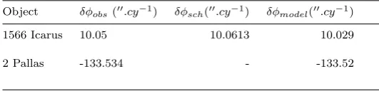
Table 2.Comparison between the observational valuesδφobsfor secular precession in units of arcsec/century and the values from the standard (Einstein) perihelion precession and the Zipoy solutionδφmodelfor selected 1566 Icarus asteroid and 2 Pallas.
Object δφobs(00.cy−1) δφsch(00.cy−1) δφmodel(00.cy−1)
1566 Icarus 10.05 10.0613 10.029
2 Pallas -133.534 - -133.52
Interestingly, the solution provides a retrograde precession besides the advanced one and the result is set by the con-served quantities and parameters initially considered. It is noteworthy to point out that the hyperbolic term persists in the result evincing the propagation of the non linear effects from the Einstein equations even with the breakage of the diffeomorphic coordinate transformations.
To obtain the correct physical units, we use the known forms for the specific orbital energy E = −GM
2γ and the specific orbital momentum L2 = µp, with µ = GM and p = γ(1−2). The terms M, γ and denote the central Sun mass, the semi-major axis and the orbital eccentricity, respectively. The Newton’s universal gravitational constant is denoted byG. Sinceβis small, the hyperbolic exponential can be approximated to e−2βπ ∼1−2βπ. It is important to stress that high orders on β are neglected. Accordingly, using eq.(43), one can obtain
δφ(zip)=− 3 2π
a2GM
c2γ3(1−2)(1−2βπ) . (44)
A more familiar expression for apsidal precession can be obtained by using the orbital period P in days in such a way we have the final form
δφ(zip)=
−6π3a2
c2(1−2)P2 (1−2βπ) , (45)
which resembles the standard Schwarzschild formula. For the physical quantities, we adopt the international sys-tem of measurement Bureau International des Poids et Mesures (Bureau International des Poids et Mesures 2006) setting one year 1yr = 365.256d, the speed of light c = 299792458m/s (Wilhelm and Dwivedi 2014; Bureau
Inter-national des Poids et Mesures 2006) and the mass of sun M = 1.98853×1030kg. The period P is given by P = T(24)(3600) and T is the sidereal orbital period in days. In the case of Mercury, we use T = 87.969 days (NASA Mercury Fact Sheet. https://nssdc.gsfc.nasa.gov).
We use 9 data points concerning observations on the perihelion advance of Mercury in units of arcsecond per cen-tury (00.cy−1) as shown in table 01. We denoteδφschfor stan-dard (Einstein) perihelion precession andδφW eylfor the re-sulting perihelion advance using the Weyl conformastatic so-lution (Capistrano, Roque and Valada, 2014), which comes from an axially-symmetric motion of a test particle in Weyl’s line element (Weyl, 1917). To control the systematics, we use GnuPlot 5.2 software to compute non-linear least-squared fitting by using the Levenberg-Marquardt algorithm for the goodness-of-fitting to data. The obtained values for the pa-rameters and the related reduced chi-squared (χ2red). Since eq.(45) has a negative sign, and to obtain an advanced pre-cession solution, we calculate its absolute value. We observed that running the parameters without any priors, we find that thea parameter has the same magnitude of the plan-etary semi-major axis as it providesa ∼ −1.15806×10¹¹, which its absolute value is roughly close to observational value of Mercury’s semi-major axis andβ= 8.86038×10⁻⁶ and the resulting value for the shift angle is 42.969600.cy−1 for aχ2red= 0.0166 and a probabilityp >0.95, which repre-sents a good fitting. It is worth noting that the negative sign for the length parameterais a relic from the hyperbolic ge-ometry that passed through the non linear effects from the initially strong gravitational field.
In table (1), the secular precession of Mercury in units of arcsec/century, comparing with standard Schwarzschild and
cylindric Weyl solutions for the perihelion shift, the obtained perihelion shiftδφZipoyreproduces closely the observed per-ihelion shift with a bonus that it naturally provides elliptical orbits which makes this solution a better physical descrip-tion for astrophysical purposes according to the shape, the topology and the symmetry aspects of the gravitational field. Departing from a spherical geometry, we are able to study precession of two asteroids. The first one corresponds to the Icarus asteroid. This asteroid is a near-Earth object (NEO) of the Apollo group with a very elliptical orbit. It has been regarded as a relativistic asteroid with an approxi-mation even close to the Sun than Mercury and also a Venus and Mars-crosser. Its observational value for the perihelion precession is 10.05 arcseconds per century with semi-major axis 1.61258×10¹¹m and a large eccentricity 0.82695 for an orbital periodT = 408.781 days (Wilhelm and Dwivedi 2014). As a result, we obtained the values for the parameters a ∼ −3.21987×10¹¹ and β = 8.0222×10⁻⁶ that provide a value for the shift angle 10.02900.cy−1 forχ2
red= 0.00272 andp >0.95.
In addition, as an example of retrograde precession, which is not accounted for Einstein standard perihelion formula, we studied the 2 Pallas protoplanet, even though the available information on 2 Pallas are still scarce. The 2 Pallas asteroid is one of the largest asteroids in asteroid belt and is a Jupiter-crosser. Its observational value for the perihelion precession is −1333.534 arcseconds per century with semi-major axis 4.14520×10¹¹mand a large eccentric-ity 0.2812 for an orbital periodT = 1686.43 days (available at http://hamilton.dm.unipi.it/astdys/index.php?pc=0, Asteroids Dynamic Site- AstDyS ). As a result, we obtained the values for the parameters a ∼ −1.680× 10¹³ and β = 8.0222×10⁻⁶ that provide a value for the shift angle
−133.48100.cy−1forχ2red= 1245.46 andp >0.95. In the two previous cases, the value of the β parameter remains the same and unless we find a counterproof, its value around
∼10−6 must remain the same for any large object in Solar system.
It reinforces the main aspect of this paper on “equiv-alence problem” in GR. As commented previously, the Weyl and Zipoy metric are asymptotically convergent to Schwarzschild coordinates but once the diffeomorphic invari-ance is not allowed, the produced gravitational fields are not the same, and they can be adjusted to a specific ending. In this case, the Zipoy seems to be a more physically appropri-ate solution as compared to the standard Einstein or PPN solution.
4 FINAL REMARKS
Our results in this paper is a fine example that the non-linearities of a system of equations imprint qualitative effects on the orbits of their solutions. We have studied solutions of vacuum Einstein’s equation of an oblate metric obtaining a set of solutions that depends on the Legendre Polynomi-als, as shown by Zipoy in his seminal paper (Zipoy 1966). In hindsight, the simplest studied solution was the so-called “monopole” solution for the zeroth order of Legendre poly-nomialsl= 0. Starting from the related Lagrange equations, we have obtained the orbit equations, which revealed to be a highly non linear equation. To obtain an analytical solution,
we have studied a closed positive infinite interval to obtain the elliptical pattern of the orbits in-between. As a result, we have obtained a non-standard expression for the perihelion precession depending on the dimensionless parameterβand the length parametera. Theβparameter was primarily fixed as a low magnitude to allow us to study the orbit equation. It is worth noting to point out that noa prioriassumptions concerning the strength of the field (as a weak field) were imposed. Moreover, the values of the length parameter a were adjust numerically using the Chi-square statistics for 9 observational data sets. We have shown the length param-eter, as posed by Zipoy, can be attributed to it a physical meaning since it is close related to semi-major axis. Interest-ingly, the values converged to the same order of magnitude of semi-major axis of Mercury. Differently from the standard Einstein’s solution and the Weyl cylindrical one, the preces-sion formula from oblate coordinates provides naturally both retrograde and advanced solutions for the perihelion preces-sion besides the fact that elliptical orbits are also native in those coordinates, which reinforces the idea that the topo-logical nature of the problem is now an important character and the strength of the gravitational field is constrained by this topology. In summary, this analysis was made in the realm of RG in a nearly newtonian limit with no need of ad-ditional extensions or modifications of the standard gravity. As future perspectives, the extended analysis of the devia-tion of light, radar echo and gravitadevia-tional lens in oblate and prolate metrics are currently in progress.
5 ACKNOWLEDGMENTS
Paola T.Z. Seidel thanks the Coordination for the Improve-ment of Higher education Personnel (Capes-Brazil) and the Funda¸c˜ao Arauc´aria/PR for the scholarship grant Capes/FA (Chamada P´ublica 19/2015). We also thank Carlos Coimbra and Rodrigo Bloot for fruitful discussions and criticisms.
REFERENCES
Anderson J.D., Keesey M.S.W., Lau E.L., Standish E.M., Newhall X.X., 1978, Acta Astronautica, 5, 4361.
Anderson J.D., Campbell J.K., Jurgens R.F., Lau E.L., Newhall X.X., Slade III M.A., Standish Jr E.M., 1992,“Recent developments in solar-system tests of gen-eral relativity”, In: H. Sato et al (Eds.): Proceedings of the 6th Marcel Grossmann Meeting on General Relativity, Kyoto, June 1991, World Scientific, Singapore, 353355. Avalos-Vargas A., Ares de Parga, G., 2012, EPJ Plus, 127,
155.
Arakida H., 2013, Int. J. Theor. Phys., 52, 5, 1408-1414. Adkins G. S.; McDonnell J., 2007, Phys. Rev. D75, 8,
082001.
Biswas A.; Mani K., 2005, Centr.Eur.Jour.Phys., 3(1), 6976.
Bureau International des Poids et Mesures, 2006. Le Syst´eme International d’Unit´es(SI), 8e ´edition, BIPM, S´evres, p. 37.
Capistrano A.J.S., Roque W.L., Valada R.S., 2014, Mon. Not. R. Astron. Soc., 444, 1639-1646.
Capistrano A.J.S., Penagos J.A.M, Al´arcon M.S., 2016, Mon. Not. R. Astron. Soc., 463, 1587-1591.
Capistrano A.J.S., Galaxies 2018, 6, 48. Cartan E., 1927, Ann. Soc. Pol. Mat 6, 1. Clemence G.M., 1964, Icarus 3, 502.
Chakraborty S., Sengupta S., 2014, Phys. Rev. D 89, 026003.
Cheung Y.K.E., Xu F., 2013, Astrophys.J., 774, 1, 65, 20. D’Eliseo M. M, 2012, Astrophys. Space Sci., 342, 1, 15-18. Deng X., Xie Y., 2014, Astrophys. Space Sci., 350, 1,
103-107.
Duncombe R.L., 1956, Astron. J. 61, 174175. Feldman M.R., 2013, PLoS ONE, 8, 11, e78114.
Gautreau R., Hoffman R.B., Armenti A., 1972, Il Nuovo Cimento B, 7(1), 71-98.
Gergerly L.A. et al., 2011, Mon. Not. R. Astron. Soc., 415, 3275-3290.
Gonz´alez G.A., Guti´errez-Pi˜neres A.C., Ospina P.A., 2008, Phys. Rev. D, 78, 064058.
Guti´errez-Pi˜neres A.C., Gonz´alez G.A., Quevedo H., 2013, Phys. Rev. D, 87, 044010.
Harko T., 2011, Mon. Not. R. Astron. Soc., 413, 4, 3095-3104.
Infeld L., Plebanski J., 1960,Motion and Relativity, Perg-amon Press.
Iorio L., 2008, Scholarly research Exchange Volume 2008, 238385.
Iorio L., 2009, A.J., 137, 3615.
Iorio L., 2009, Int. J. Mod. Phys. D18, 947. Iorio L., 2005, Class.Quant.Grav., 22, 24,5271-5281. Iorio L., 2006, JCAP, 05, 002.
Iorio L., 2008, Advances in Astronomy, 268647.
Iorio L. et al., 2011, Astrophys. Space Sci., 331, 2, 351-395. Jalalzadeh S. et al., 2009, Class.Quant.Grav., 26, 155007. Karlhede A., 1980, Gen. Rel. Grav., 12, 693-707.
Li Z. et al., 2014, RAA, 14, 2, 139-143.
Lim P.H., Wesson P.S., 1992, Astrophys.J., 397, L91-L94. Mak M.K., Harko T., 2004, Phys.Rev.D70, 024010. Maia M.D.; Capistrano, A.J.S.; Muller D., 2009, IJMPD,
18, 1273-1289.
Misner C., Thorne K.S., Wheeler J.A., 1973,Gravitation, W.H. Freeeman & Co.
Morton D.C., 1956, J.R. Astron. Soc. Canada 50, 223. Nambuya G.G., 2010, Mon. Not. R. Astron. Soc., 403, 1381. Nobili A.M., Will C.M., 1986, Nature, 320, 39-41.
Pitjeva E. V., Pitjev N.P., 2013, Mon. Not. R. Astron. Soc., 432, 4, 3431-3437.
Pitjev N. P., Pitjeva, E. V., 2013, Astron. Lett., 39, 3, 141-149.
Rosen N., 1949, Rev. Mod. Phys., 21, 503.
Ruggiero M. L., 2014, Int. J. Mod. Phys. D23, 5, 1450049. Schmidt H.J., 2008, Phys. Rev.D 78, 023512.
Shapiro I.I., Pettengill G.H., Ash M.E., Ingalls R.P., Campbell D.B., Dyce R.B., 1972, Phys. Rev. Lett., 28, 15941597.
Shapiro I.I, Counselman III C.C., King R.W., 1976, Phys. Rev. Lett., 36, 555585.
Shapiro, I.I., 1990, “Solar system tests of general relativ-ity: Recent results and present plan”, In: N. Ashby et al (Eds.): General Relativity and Gravitation, 1989, Pro-ceedings of the 12th International Conference on General
Relativity and Gravitation, Cambridge University Press, Cambridge, 313330.
Stephani H., Kramer D., MacCallum M., Hoenselaers C., Herlt E., 2003,Exact Solutions of Einstein’s Field Equa-tions. Cambridge: Cambridge University Press.
Wilhelm K., Dwivedi B. N., 2014, New Astronomy, 31, 51-55.
Ujevic M., Letelier P.S., 2004, Phys. Rev. D, 70, 084015. Ujevic M., Letelier P.S., 2007, Gen.Rel.Grav., 39,
1345-1365.
Vogt D., Letelier, P.S., 2008, Mon. Not. R. Astron. Soc., 384, 834-842.
Weyl H., 1917, Ann. Phys., 359, 117.
Will C.M., 2006, Living Rev. Relativity 9, 3, URL (accessed 29 May 2018).
Wilhelm K., Dwivedi B. N., 2014, New Astronomy, 31, 51-55.
Zipoy M.D., 1966, Jour. Math. Phys., 7, 1137.
Yamada K., Asada H., 2012, Mon. Not. R. Astron. Soc., 423, 3540-3544.