Graph-Induced Multilinear Maps from Lattices
Craig Gentry IBM
Sergey Gorbunov∗ MIT
Shai Halevi IBM
November 11, 2014
Abstract
Graded multilinear encodings have found extensive applications in cryptography ranging from non-interactive key exchange protocols, to broadcast and attribute-based encryption, and even to software obfuscation. Despite seemingly unlimited applicability, essentially only two candidate constructions are known (GGH and CLT). In this work, we describe a new graph-induced multilinear encoding scheme from lattices. In a graph-graph-induced multilinear encoding scheme the arithmetic operations that are allowed are restricted through an explicitly defined directed graph (somewhat similar to the “asymmetric variant” of previous schemes). Our construction encodes Learning With Errors (LWE) samples in short square matrices of higher dimensions. Addition and multiplication of the encodings corresponds naturally to addition and multiplication of the LWE secrets.
∗
Contents
1 Introduction 1
1.1 Our Results . . . 1
1.1.1 Our Techniques . . . 2
1.2 Applications . . . 3
1.3 Organization . . . 4
2 Preliminaries 5 2.1 Lattice Preliminaries . . . 5
2.1.1 Gaussian Distributions . . . 5
2.1.2 Trapdoors for Lattices . . . 6
2.1.3 Leftover Hash Lemma Over Gaussians . . . 6
2.2 Graded Multilinear Encodings . . . 6
2.2.1 Syntax of Graph-Induced Graded Encoding Schemes . . . 7
2.2.2 Correctness . . . 8
2.2.3 Variations . . . 9
3 Our Graph-Induced Multilinear Maps 9 3.1 Correctness . . . 11
3.2 A Commutative Variant . . . 12
3.3 Public Sampling and Some Other Variations . . . 13
4 Cryptanalysis 13 4.1 Encoding of Zero is a Weak Trapdoor . . . 14
4.2 Recovering HiddenAv’s. . . 15
5 Applications 17 5.1 Multipartite Key-Agreement . . . 17
5.2 Candidate Branching-Program Obfuscation . . . 19
5.2.1 A Concrete BP-Obfuscation Candidate . . . 21
Bibliography 22
1
Introduction
Cryptographic multilinear maps are an amazingly powerful tool: like homomorphic encryption schemes, they let us encode data in a manner that simultaneously hides it and permits processing on it. But they go even further and let us recover some limited information (such as equality) on the processed data without needing any secret key. Even in their simple bi-linear form (that only supports quadratic processing) they already give us pairing-based cryptography [Jou04, SOK00, BF03], enabling powerful applications such as identity- and attribute-based
encryption [BF01, Wat05, GPSW06], broadcast encryption [BGW05] and many others. In
their general form, cryptographic multilinear maps are so useful that we had a body of work examining their applications even before we knew of any candidate constructions to realize them [BS03, RS09, PTT10, Rot13].
Formally, a non-degenerate map between order-q algebraic groups, e : Gd → GT, is
d−multilinear if for alla1, . . . , ad∈Zq and g∈G,
e(ga1, . . . , gad) =e(g, . . . , g)a1·...·ad.
We say that the mapeis “cryptographic” if we can evaluate it efficiently and at least the discrete-logarithm in the groups G, GT is hard.
In a recent breakthrough, Garg, Gentry and Halevi [GGH13b] gave the first candidate construction of multilinear maps from ideal lattices, followed by a second construction by Coron, Lepoint and Tibouchi [CLT13] over the integers. (Some optimizations to the GGH scheme were proposed in [LSS14]). Due to certain differences between their construction and “ideal” multilinear maps, Garg et al. (and Coron et al.) called their constructions “graded encoding schemes.” These graded encoding schemes realize an approximate version of multilinear maps with no explicit algebraic groups, where the transformation a 7→ ga is replaced by some (randomized) encoding function.
Moreover, these constructions are “graded”, in the sense that they allow intermediate computation. One way to think of these intermediate computations is as a sequence of levels (or groups)G1, . . . , Gdand a set of mapseij such that for allgai ∈Gi, gbj ∈Gj (satisfyingi+j≤d),
eij(gai, gbj) =gabi+j.Asymmetric variant of graded multilinear maps provides additional structure on
how these encodings can be combined. Each encoding is assigned with a set of levels S ⊆ [N]. Given two encodingsgSa, gSb0 the map allows to compute gSab∪S0 only if S∩S0 =∅.
Both [GGH13b] and [CLT13] constructions begin from some variant of homomorphic encryption and use public-key encryption as the encoding method. The main new ingredient, however, is that they also publish a defective version of the secret key, which cannot be used for decryption but can be used to test if a ciphertext encrypts a zero. (This defective key is called the “zero-test parameter”.) Over the last two years, the applications of (graded) multilinear maps have expanded much further, supporting applications such as witness encryption, general-purpose obfuscation, functional encryption, and many more [GGSW13, GGH+13c, GGH+13a, BGG+14, BZ14].
1.1 Our Results
construction of graph-induced multilinear maps does not rely on ideal lattices or hard-to-factor integers. Rather,we use standard random latticessuch as those used in LWE-based cryptography. We follow a similar outline to the previous constructions, except our instance generation algorithm takes as input a description of a graph. Furthermore, our zero-testerdoes not include any secrets about the relevant lattices. Rather, in our case the zero-tester is just a random matrix, similar to a public key in common LWE-based cryptosystems.
Giving up the algebraic structure of ideal lattices and integers could contribute to a better understanding of the candidate itself, reducing the risk of unforeseen algebraic crypt-analytical attacks. On the flip side, using our construction is sometimes harder than previous construction, exactly because we give up some algebraic structure. For that same reason, we were not able so far to reduce any of our new construction to “nice” hardness assumptions, currently they are all just candidate constructions, that withstood our repeated cryptanalytic attempts at breaking them. Still we believe that our new construction is a well needed addition to our cryptographic toolbox, providing yet another avenue for implementing multilinear maps.
1.1.1 Our Techniques
Our starting point is the new homomorphic encryption (HE) scheme of Gentry, Sahai and Waters [GSW13]. The secret key in that scheme is a vectora∈Zm
q , and a ciphertext encryptingµ∈Zq is
a matrixC∈Zm×m
q with small entries such thatC·a=µ·a+efor some small error vectore. In
other words, valid ciphertexts all have the secret key a as an “approximate eigenvector”, and the eigenvalue is the message. Given the secret eigenvectora, decoding arbitrary µ’s becomes easy.
This HE scheme supports addition and multiplication, but we also need a public equivalent of the approximate eigenvector for zero-testing. The key idea is to replace the “approximate eigenvector” with an “approximate eigenspace” by increasing the dimensions. Instead of having a single approximate eigenvectors, our “approximate eigenspace” is described bynvectorsA∈Zmq×n.
The approximate eigenvalues will not merely be elements ofZq, but rather matricesS∈Znq×nwith
small entries. An encoding of S is a matrixC∈Zm×m with small entries such that
C·A=A·S+E
for small noise matrixE∈Zmq×n. In other words,Cis a matrix that maps any column vector inA
to a vector that is very close to the span of A. In that sense,A is an approximate eigenspace. In the HE scheme,a was a secret key that allowed us to easily recoverµ. However, for the eigenspace setting, assumingAis just a uniformly random matrix and S is a random small matrix, A·S+E is an LWE instance that looks uniform even when givenA.
Overview of Our Construction. Our construction is parametrized by a directed acyclic graph
G = (V, E). For each node v ∈ V, we assign a random matrix Av ∈ Zmq×n. Any path u ; v
(which can be a single edge) can be assigned with an encodingD∈Zm×m
q of some plaintext secret
S∈Znq×n satisfying
D·Au =Av·S+E (1)
for some small errorE∈(χ)m×n.
given encodings D1,D2 at pathu;v, we have that:
(D1+D2)·Au ≈ Av·S1+Av·S2 = Av·(S1+S2).
Multiplication of encodings can only be performed when they form a complete path. That is, given encodingsD1 and D2 relative to paths u;v andv;w respectively, we have:
D2·D1·Au = D2·(Av·S1+E1)
= (Aw·S2+E2)·S1+D2·E1 = Aw·S2·S1+E2·S1+D2·E1
| {z }
E0
(2)
whereE0 is small since the errors and matricesS1,D2 have small entries. Furthermore, it is possible
to compare two encodings with the same sink node. That is, given D1 and D2 relative to paths
u; v and w; v, it is sufficient to check if D1·Au−D2·Aw is small since if S1 =S2, then we
have
D1·Au−D2·Aw = (Av·S1+E1)−(Av·S2+E2) = E1−E2 (3)
Hence, the random matricesAu,Aw∈Zq, which are commonly available in the public parameters,
is sufficient for comparison and zero-testing.
As we explain in Section 3, generating the encoding matrices requires knowing a trapdoor for the matrices Ai. But for the public-sampling setting, it is possible to generate encodings of many
random matrices during setup, and later anyone can take a random linear combinations of them to get “fresh” random encodings.
We remark that since S needs to be small in Eqn. (2), our scheme only supports encoding of small plaintext elements, as opposed to arbitrary plaintext elements as in previous schemes.1 Another difference is that in the basic construction our plaintext space is a non-commutative ring (i.e. square matrices). We extend to the commutative setting in Section 3.2.
Variations and parameters. We also describe some variations of the basic scheme above, aimed at improving the parameters or offering different trade-offs. One standard way of improving parameters is to switch to a ring-LWE setting, where scalars are taken from a large polynomial ring (rather than being just integers), and the dimension of vectors and matrices is reduced proportionally. In our context, we can also use the same approach to move to a commutative plaintext space, see Section 3.2.
1.2 Applications
Our new constructions support many of the known cryptographic uses of graded encoding. Here we briefly sketch two of them.
1The only exception is that the leftmost plaintext matrixSin a product could encode a large element, as Eqn. (2)
is not affected by the size ofS1. Similarly the rightmost encoding matrixDin a product need not be small. We do
Non-interactive Multipartite Key-Exchange. Consider k-partite key-exchange. We design a graph in a star topology with k-branches each of length k−1 nodes. All branches meet at the common sink node A0. For each branch i, we associate encodings of small LWE secrets
t1, . . . , . . . , tk in a specific order. The public parameters consists of many such plaintext values tis
and their associated encodings. Each playerjtakes a random linear combination of these encodings. It stores one of the encodings along the path as the secret key and broadcasts the rest of to other players. Assume some canonical ordering of the players. Each player computes thek−1 product of the other players’ encodings along the path with index j and its own secret encoding. This yields an encodingD of T∗ =Q
i∈[k]si, satisfying
D·Aj,1=A0·
Y
i∈[k]
si+ noise
And the players obtain the shared secret key by applying a randomness extractor on the most significant bits.
Branching-program obfuscation. Perhaps the “poster application” of cryptographic graded encodings is to obtain general-purpose obfuscation [GGH+13c, BR14a, BGK+14, PST14, GLSW14],
with the crucial step being the use of graded encoding to obfuscate branching programs. These branching programs are represented as a sequence of pairs of encoded matrices, and the user just picks one matrix from each pair and then multiply them all in order.
This usage pattern of graded encoding fits very well into our graph-induced scheme since these matrices are given in a pre-arranged order. We describe a candidate obfuscation construction from our multilinear map based on a path graph. Informally, to obfuscate a length-Lmatrix branching program {Bi,b}, we first perform Kilian’s randomization and then encode values R−i−11Bi,0Ri and
R−i−11Bi,1Ri relative to the edgei. The user can then compute an encoding of a product of matrices
corresponding to its input. If the product Q
i∈[L]Bi,xvari =I, then the user obtains an encoding D satisfying:
D·A0 =AL·I+noise
GivenAL·I+noise0in the public parameters (or its encoding), the user can then learn the result of
the computation by a simple comparison. We note that our actual candidate construction is more involved as we deploy additional safeguards from the literature (See Section 5.2).
1.3 Organization
In Section 2, we provide some background and present the syntax of graph-induced multilinear maps. In Section 3, we describe our basic construction in the non-commutative variant. In Subsection 3.2 we show how to extend our basic construction to commutative variant. In Section 4, we analyze the security of our construction. In Section 5 we present applications of our construction to key-exchange and obfuscation.
2
Preliminaries
Notation. For any integerq≥2, we letZqdenote the ring of integers moduloq and we represent Zq as integers in (−q/2, q/2]. We let Zqn×m denote the set of n×m matrices with entries in Zq.
We use bold capital letters (e.g. A) to denote matrices, bold lowercase letters (e.g. x) to denote vectors.
If A1 is ann×mmatrix andA2 is ann×m0 matrix, then [A1|A2] denotes the n×(m+m0)
matrix formed by concatenating A1 and A2. Similarly, if A1,A2 have dimensions n×m and A2
is ann0×m, respectively, then we denote by (A1/A2) the (n+n0)×m matrix formed by putting
A1 on top ofA2. Similar notations apply to vectors. When doing matrix-vector multiplication we
usually view vectors as column vectors.
A functionf(n) isnegligibleif it iso(n−c) for allc >0, and we use negl(n) to denote a negligible function of n. We say thatf(n) is polynomialif it isO(nc) for somec >0, and we use poly(n) to denote a polynomial function ofn. An event occurs with overwhelming probabilityif its probability is 1−negl(n). The notationbxedenotes the nearest integer tox, rounding toward 0 for half-integers. The `∞ norm of a vector is denoted by kxk = maxi|xi|. We identify polynomials with their
representation in some standard basis (e.g., the standard coefficient representation), and the norm of a polynomial is the norm of the representation vector. The norm of a matrix, kAk, is the norm of its largest column.
Extractors. An efficient (n, m, `, )-strong extractor is a poly-time algorithmExtract:{0,1}n→ {0,1}` such that for any random variable W over {0,1}n with min-entropy m, it holds that the
statistical distance between (Extractα(W), α) and (U`, α) is at most. Here,α denotes the random
bits used by the extractor. Universal hash functions [CW79, WC81] can extract`=m−2 log1+ 2 nearly random bits, as given by the leftover hash lemma [HILL99]. This will be sufficient for our applications.
2.1 Lattice Preliminaries
2.1.1 Gaussian Distributions
For a real parameter σ > 0, define the spherical Gaussian function on Rn with parameter σ
as ρσ(x) = exp(−π||x||n/σ2) for all x ∈ Rn. This generalizes to ellipsoid Gaussians, where we
replace the parameter σ ∈ R by the (square root of the) covariance matrix Σ ∈ Rn×n: For a
rank-n matrix S ∈ Rm×n, the ellipsoid Gaussian function on Rn with parameter S is defined by
ρS(x) = exp(−πxT(STS)−1x) for all x ∈ Rn. The ellipsoid discrete Gaussian distribution with
parameter S over a set L⊂Rn is D
L,S(x) = ρS(x)/ρS(L), where ρS(L) denotes
P
x∈LρS(x) and
serves as just a normalization factor. The same notations also apply the to spherical case,DL,σ(·),
and in particularDZn,r denotes the n-dimensional discrete Gaussian distribution.
It follows from [MR07] that whenLis a lattice andσ is large enough relative to its “smoothing parameter” (alternatively its λn or the Gram-Schmidt norm of one of its bases), then for every
point c∈Rn we have
Prkx−ck> σ√n:x←R DL,σ,c
≤ negl(n).
Also under the same conditions, the probability for a random sample from DZm,σ to be 0 is
2.1.2 Trapdoors for Lattices
Lemma 2.1 (Lattice Trapdoors [Ajt99, GPV08, MP12]). There is an efficient randomized algorithm TrapSamp(1n,1m, q) that, given any integers n ≥ 1, q ≥ 2, and sufficiently large
m = Ω(nlogq), outputs a parity check matrix A ∈Zmq×n and some ‘trapdoor information’ τ that
enables sampling small solutions to rA=u (modq).
Specifically, there is an efficient randomize algorithm PreSample such that for large enough
s= Ω(√nlogq)and with overwhelming probability over(A, τ)←TrapSamp(1n,1m, q), the following two distributions are withinnegl(n) statistical distance:
• D1[A, τ]chooses a uniform u∈Zn
q and uses τ to solve for rA=u (modq),
D1[A, τ] def=
(u,r) : u←Znq; r←PreSample(A, τ,u, s) .
• D2[A] chooses a Gaussianr←DZm,s and sets u:=rAmodq,
D2[A] def= {(u,r) : r←DZm,s; u:=rAmodq}.
We can extendPreSamplefrom vectors to matrices by running it ktimes onkdifferent vectors u and concatenating the results, hence we writeR←PreSample(A, τ,U, s).
We also note that any small-enough full rank matrix T (over the integers) such that TA = 0 (modq) can be used as the trapdoorτ above. This is relevant to our scheme because in many cases an “encoding of zero” can be turned into such a trapdoor (see Section 4).
2.1.3 Leftover Hash Lemma Over Gaussians
Recent works [AGHS13, AR13] considered the setting where the columns of a matrixX∈Zt×kare
drawn independently from a “wide enough” Gaussian distribution over a latticeL⊂Zt,x
i ←DL,S.
Once these columns are fixed, we consider the distribution DX,σ, induced by choosing an integer vector r from a discrete spherical Gaussian over Zt with parameter σ and outputting y = XTr, DX,σ := {XTr : r ← DZt,σ}. It turns out that with high probability over the choice of X,
the distribution DX,σ is statistically close to ellipsoid GaussianDL,σX (and moreover the singular values ofX are of size roughly σ√t).
Theorem 2.2 ([AGHS13, AR13]). For integers k ≥ 1, t = poly(k), σ = Ω(plog(k/)) and σ0 = ˜
Ω(kσplog(1/)), we have that with probability 1−2−k over the choice X ← (D
Zk,σ)
t that the
statistical distance between DX,σ0 andD
Zk,σ0XT is smaller than .
2.2 Graded Multilinear Encodings
2.2.1 Syntax of Graph-Induced Graded Encoding Schemes
There are several variations of graded-encoding systems in the literature, such as public/secret encoding, with/without re-randomization, symmetric/asymmetric, etc. Below we define the syntax for our scheme, which is still somewhat different than all of the above. The main differences are that our encodings are defined relative to edges of a directed graph (as opposed to levels/sets/vectors as in previous schemes), and that we only encode “small elements” from the plaintext space. Below we provide the relevant definitions, modifying the ones from [GGH13b].
Definition 2.1(Graph-Induced Encoding Scheme). A graph-based graded encoding scheme with se-cret sampling consists of the following (polynomial-time) procedures,Ges= (PrmGen,InstGen,Sample,
Enc,add,neg,mult,ZeroTest,Extract):
• PrmGen(1λ, G,C): The parameter-generation procedure takes the security parameter λ, under-lying directed graph G = (V, E), and the class C of supported circuits. It outputs some global parameters of the system gp, which includes in particular the graph G, a specification of the plaintext ringR and also a distribution χ over R.
For example, in our case the global parameters consists of the dimension n of matrices, the modulusq and the Gaussian parameter σ.
• InstGen(gp): The randomized instance-generation procedure takes the global parametersgp, and outputs the public and secret parameters sp,pp.
• Sample(pp): The sampling procedure samples an element in the the plaintext space, according to the distributionχ.
• Enc(sp, p, α): The encoding procedure takes the secret parameters pp, a path p=u ; v in the graph, and an elementα∈Rfrom the support of theSampleprocedure, and outputs an encoding
up of α relative to p. 2
• neg(pp, u), add(pp, u, u0),mult(pp, u, u0). The arithmetic procedures are deterministic, and they all take as input the public parameters and use them to manipulate encodings.
Negation takes an encoding of α∈R relative to some path p=u;v and outputs encoding of
−α relative to the same path. Addition takes u, u0 that encode α, α0 ∈ R relative to the same path p, and outputs an encoding of α+α relative to p. Multiplication takes u, u0 that encode
α, α0 ∈R relative to consecutive paths p=u ; v and p0 =v ;w, respectively. It outputs an encoding of α·α0 relative to the combined path u;w.
• ZeroTest(pp, u): Zero testing is a deterministic procedure that takes the public parameters pp
and an encoding u that is tagged by its path p. It outputs 1 if u is an encoding of zero and 0 if it is an of a non-zero element.
• Extract(pp, u): The extraction procedure takes as input the public parametersppand an encoding
u that is tagged by its path p. It outputs a λ-bit string that serves as a “random canonical representation” of the underlying plaintext element α (see below).
2
2.2.2 Correctness
The graphG, in conjunction with the procedures for sampling, encoding, and arithmetic operations, and the class of supported circuits, implicitly define the setSGof “valid encodings” and its partition
into setsSG(α) of “valid encoding of α”.
Namely, we consider arithmetic circuits whose wires are labeled by paths in G in a way that respects the permitted operations of the scheme (i.e., negation and addition have all the same labels, and multiplication has consecutive input paths and the output is labeled by their concatenation). Then SG consists of all the encoding that can be generated by using the sampling/encoding
procedures to sample plaintext elements and compute their encoding, then compute the operations of the scheme according to Π, and collect the encoding at the output of Π. An encoding u ∈SG
belongs to SG(α) is there exists such circuit Π and inputs for which Π outputsα when evaluated on plaintext elements. Of course, to be useful we require that the setsSG(α) form a partition of SG.
We can also sub-divide each SG(α) intoSp(α) for different pathsp in the graph, depending on the
label of the output wire of Π (but here it is not important that these sets are disjoint), and define
Sp =Sα∈RS (α) p .
Note that the sets Sp(α) can be empty, for example in our construction the sampling procedure
only outputs “small” plaintext valuesα, so a “large” β would haveSp(β)=∅. Below we denote the
set of α’s with non-empty encoding sets (relative to path p) by SMALLp def
= {α ∈R : Sp(α) 6= ∅},
and similarly SMALLG def
= {α∈R:SG(α)6=∅}.
We assume for simplicity that the setsSMALLdepend only on the global parameters gpand not the specific parameters sp, pp. (This assumption holds for our construction and it simplifies the syntax below.)
We can now state the correctness conditions for zero-testing and extraction. For zero-testing we require that ZeroTest(pp, u) = 1 for every u ∈ S(0) (with probability one), and for every
α ∈ SMALLG, α 6= 0 it holds with overwhelming probability over instance-generation that
ZeroTest(pp, u) = 0 for every encoding u∈SG(α).
For extraction,we roughly require that Extract outputs the same string on all the encodings of the same α, different strings on encodings of different α’s, and random strings on encodings of “randomα’s.” Formally, we require the following for any global parametersgpoutput byPrmGen:
• For any plaintext element α ∈ SMALLG and path p in G, with overwhelming probability
over the parameters (sp,pp) ← InstGen(gp), there exists a single value x ∈ {0,1}λ such that
Extract(pp, u) =x holds for allu∈Sp(α).
• For any α 6= α0 ∈ SMALLG and path p in G, it holds with overwhelming probability over
the parameters (sp,pp) ← InstGen(gp) that for any u ∈ Sp(α) and u0 ∈ S(α
0)
p , Extract(pp, u) 6=
Extract(pp, u0).
• For any path p in G and distribution D over SMALLp with min-entropy 3λ or more, it holds
with overwhelming probability over the parameters (sp,pp) ← InstGen(gp) that the induced distribution{Extract(pp, u) :α← D, u∈Sd(α)}is nearly uniform over {0,1}λ.
2.2.3 Variations
Public sampling of encoded elements. One useful variation allows a public sampling procedure that takes as input pp rather than spand outputs both a plaintext α and its encoding
up relative to some pathp. In many cases it is easy to go from secret-encoding to public sampling.
Specifically, given a scheme that supports secret encoding we can augment the instance-generation procedure by sampling many tuples (αi, ui) relative to relevant paths (e.g., the edges in G) and
adding them to the public parameters. Then a public sampling procedure can just use a subset sum of these tuples as a new sample, which would have some other distributionχ0.
If the distribution χof the secret sampling procedure was uniform overR, then by the leftover hash lemma so is the distributionχ0 of the public sampling procedure. Similarly, ifχwas a Gaussian then using the Gaussian leftover-lemma Theorem 2.2 alsoχ0 is a Gaussian (with somewhat different parameters).
In our construction we have a Gaussian distribution χ, so we can use this method to transform our scheme to one with a public sampling procedure.
Re-randomization. In some cases one may want to re-randomize a given encoding with changing the encoded value or the path in G, or to compute given a plaintext element the corresponding encoding relative to come path. Our construction does not support re-randomization (see Section 4).
3
Our Graph-Induced Multilinear Maps
The plaintext space in our basic scheme is the non-commutative ring of matrices R=Znq×n, later
in Section 3.2 we describe a commutative variant. In this section we only deal with correctness of these schemes, their security is discussed in Section 4.
As sketched in the introduction, for the basic scheme we have an underlying directed acyclic graph G = (V, E), we identify a random matrix Av ∈ Zqm×n with each node v ∈ V, and
encodings in the scheme are defined relative to paths. A small plaintext matrix S∈R is encoded wrt to the path u ; v via another small matrix D ∈ Zqm×m such that D · Au ≈ Av ·S.
In more detail, we have the following graded encoding scheme Ges = (PrmGen,InstGen,Sample,
Enc,add,neg,mult,ZeroTest,Extract):
• PrmGen(1λ, G,C): On input the security parameter λ, an underlying DAG G = (V, E), and classC of supported circuits, we compute:
1. LWE parametersn, m, q and error distribution χ=DZ,s.
2. A Gaussian parameters σ forPreSample.
3. Another parametertfor the number of most significant bits used for zero-test and extraction.
The constraints that dictate these parameters are described in Appendix A. The resulting parameters for a DAG of diameter d are n = Θ(dλlog(dλ)), q = (dλ)Θ(d), m = Θ(ndlogq),
s=√n,σ =pn(d+ 1) logq, and t=b(logq)/4c −1. These global parameters gp(including the graphG) are given to all the procedures below.
1. Use trapdoor-sampling to generate|V|matrices with trapdoors, one for each node.
∀v∈V, Av, τv
←TrapSamp(1n,1m, q)
2. Choose the randomness-extractor seedβ from a pairwise-independent function family, and a uniform “shift matrix”∆∈Zmq×n.
The public parameters arepp:= {Av :v ∈V}, β,∆
and the secret parameters include also the trapdoors {τv :v∈V}.
• Sample(pp): This procedure just samples an LWE secretS←(χ)n×n as the plaintext.
• Enc(sp, p,S): On input the matricesAu,Av, the trapdoorτu, and the small matrixS, sample
an LWE error matrixEi ←(χ)m×n, setV=Av·S+E∈Zmq×n, and then use the trapdoorτu
to compute the encoding Dp s.t. Dp·Au =V,Dp ← PreSample(Au, τu,V, σ). The output is
the plaintextS and encodingDp.
• The arithmetic operations are just matrix operations inZmq×m:
neg(pp,D) :=−D, add(pp,D,D0) :=D+D0, and mult(pp,D,D0) :=D·D0.
To see that negation and addition maintain the right structure, let D,D0 ∈ Zmq×m be two
encodings reltive to the same pathu;v. NamelyD·Au =Av·S+EandD0·Au=Av·S0+E0,
with the matricesD,D0,E,E0,S,S0 all small. Then we have
−D·Au = Av·(−S) + (−E),
and (D+D0)·Au = (Av·S+E) + (Av·S0+E0) = Av·(S+S0) + (E+E0),
and all the matrices−D,−S,−E, D+D0, S+S0, E+E0 are still small. For multiplication, consider encodings D,D0 relative to pathsv;w and u;v, respectively, then we have
(D·D0)·Au = D· Av·S0+E0
= Aw·S+E
·S0+D·E0 = Aw·(S·S0) + (E·S0+D·E0)
| {z }
E00
,
and the matricesD·D0,S·S0, and E00 are still small.
Of course, the matricesD,S,E all grow with arithmetic operations, but our parameter-choice enures that for any encoding relative to any path in the graph u;v (of length≤d) we have D·Au =Av·S+E whereE is still small, specifically kEk< q3/4≤q/2t+1.
• ZeroTest(pp,D). Given an encodingDrelative to pathu;vand the matrixAu, our zero-test
procedure outputs 1 if and only ifkD·Auk< q/2t+1.
• Extract(pp,D): Given an encoding D relative to path u ;v, the matrix Au and shift-matrix
∆, and the extrator seedβ, we computeD·A0+∆, collect thetmost-significant bits from each
entry (when mapped to the interval [0, q−1]), and apply the randomness extractor, outputting
w:=RandExtβ msbt(D·Au+∆)
3.1 Correctness
Correctness of the scheme follows from our invariant, which says that encoding of some plaintext matrixS relative to any pathu;v of legnth≤dsatisfies D·Au=Av·S+E forkEk< q/2t+1.
Correctness of Zero-Test. An encoding of zero satisfiesD·Au =E, hencekD·Auk< q/2t+1.
On the other hand, sinceAv is uniform then for any nonzero S we only get kAv·Sk ≤q/2t with
exponentially small probability, and since kEk< q/2t+1 then
kD·Auk ≥ kAv·Sk − kEk> q/2t−q/2t+1 ≥q/2t+1.
Hence with overwhelming probability over the choise ofAv, our zero-test will output 0 onall the
encoding ofS.
Correctness of Extraction. We begin by proving that for any plaintext matrix S and any encoding D of S (relative to u; v), with overwhelming probability over the parameters we have thatmsbt(D·Au+∆) =msbt(Av·S+∆).
Since the two matrices M=Av·S+∆and M0=D·Au+∆differ in each entry by at most
q/2t+1 modulo q, they can only differ in their top t bits due to the mod-q reduction, i.e., if for some entry we have [M]k,` ≈ 0 but [M0]k,` ≈ q or the other way around. (Recall that here we
reduce mod-q into the interval [0, q−1].) Clearly, this only happens whenM≈M0 ≈0 (modq), in particular we need
−< q/2t+1<[AvS+∆]k,`< q/2t+1.
For any S and Av, the last condition occurs only with exponentially small probability over the
choise of∆. We conclude that if all the entries of|Av·S+∆|are larger than q/2t+1 (moduloq),
which happens with overwhelming probability, then for all level-iencodings Dof S, the topt bits of D·Au agree with the top t bits ofAv ·S. We call a plaintext matrix S “v-good” if the above
happens, and denote their set by GOODv. With this notation, the arguments above say that for
any fixed S, v, we have S ∈ GOODv with overwhelming probability over the instance-generation
randomness.
Same input implies same extracted value. For any plaintext matrix S ∈GOODv, clearly all
its encodings relative to u ; v agree on the top t bits of D·Au (since they all agree with
Av·S). Hence they all have the same extracted value.
Different inputs imply different extracted values. IfD,D0 encode different plaintext matri-ces thenD−D0is an encoding of non-zero, hencek(D−D0)·Auk q/2texcept with negligible
probability, D·Au+∆ and D0·Au+∆must differ somewhere in their top t bits. Since we
use universal hashing for our randomness extractor, then with high probability (over the hash functionβ) we getRandExtβ msbt(D·Au+∆)
6
=RandExtβ msbt(D0·Au+∆)
.
Random input implies random extracted value. Fix some high-entropy distributionDover inputsS. Since for every S we have Pr[S∈GOODv] = 1−negl(λ) then also with overwheling
probability over the parameters we have PrS←D[S ∈ GOODv] = 1−negl(λ). It is therefore
We observe that the functionH(S) =Av·S+∆is itself pairwise independent on each column
of the output separately, and therefore so is the functionH0(S) =msbt(H(S)). 3 We note that
H0 has very low collision probability, its range has many more than 6λbits in every column, so for every S6=S0 we get PrH0[H0(S) =H0(S0)]2−6λ. Therefore H0 is a good condenser, i.e., if the min-entropy ofD is above 3λ, then with overwhelming probability over the choise of H, the min-entropy ofH0(D) is above 3λ−1 (say). By the extraction properties ofRandExt, this implies thatRandExtβ(H0(D)) is close to uniform (whp overβ).
3.2 A Commutative Variant
In some applications it may be convenient or even necessary to work with a commutative plaintext space. Of course, simply switching to a commutative sub-ring of the ring of matrices (such ass·I
for a scalarsand the identityI) would be insecure, but we can make it work by moving to a larger ring.
Cyclotomic rings. We switch from working over the ring of integers to working over polynomial rings, R=Z[x]/(F(X)) andRq =R/qR for some degreen irreducible integer polynomialF(X)∈ Z[X] and an integer q ∈Z. Elements of this ring correspond to degree-(n−1) polynomials, and
hence they can be represented byn-vectors of integers in some convenient basis. The norm of a ring element is the norm of its coefficient vector, and this can be extended as usual for norm of vectors and matrices overR. Addition and multiplication are just polynomial addition and multiplication modulo F(X) (and also moduloq when talking about Rq).
As usual, we need a ring where the norm of a product is not much larger than the product of the norms, and this can be achieved for example by using F = ΦM(X), the M’th cyclotomic
polynomial (of degreen=φ(M)). All the required operations and lemmas that we need (such as trapdoor and pre-image sampling etc.) can be extended also to this setting, see e.g. [LPR13].
The construction remains nearly identical, except all operations are now performed over the ringsRandRq and the dimensions are changed to match. We now have the “matrices”Av ∈Rmq×1
with only one column (and similarly the error matrices are E ∈ Rmq×1), and the plaintext space is Rq itself. An encoding of plaintext element s ∈ Rq relative to path u ; v is a small matrix
D∈Rmq×m such that
D·Au=Av·s+E
where E0 is some small error term. As before, we only encode small plaintext elements, i.e., the sampling procedure draws s from a Gaussian distribution with small parameter. The operations all remain the same as in the basic scheme.
We emphasize that it is the plaintext space that is commutative, not the space of encoding. Indeed, if we haveD,D0 that encode s, s0 relative to pathsv ;w and u;v, respectively, we can only multiply them in the order D·D0. Multiplying in the other order is inconsistent with the graph G and hence is unlikely to yield a meaningful result. What makes the symmetric scheme useful is the ability to multiply the plaintext elements in arbitrary order. For example for D,D0 that encodes, s0 relative to pathsu;wandv;w, we can compute eitherD·Au·s0 orD0·Av·s
and the results will both be closeAv·ss0 (and hence also close to each other).
3Ifqis not a power of two thenH0
3.3 Public Sampling and Some Other Variations
As mentioned in Appendix 2.2.1, we can provide a public sampling procedure relative to any desired path p = u ; v by publishing with the public parameters a collection of pairs generated by the secret sampling procedure above, {(Sk,Dk) : k= 1, . . . , `} (for some large enough `). The public
sampling procedure then takes a random linear combination of these pairs as a new sample, namely it chooses r←DZ`,σ0 and compute the encoding pair as:
(S,D) :=
X
i∈[`]
riSi ,
X
i∈[`]
riDi
.
It is easy to see that the resulting D encodes S relative to the edge e. Also by Theorem 2.2, the plaintext matrixS is distributed according to a Gaussian distribution whp.
We note that in most applications it is not necessary to include in the public parameters the matrices for all the nodes in the graph. Indeed we typically only need the matrices for the source nodes in the DAG in order to preform zero-testing or extraction.
Some Safeguards. Since our schemes are graph-based, and hence the order of products is known in advance, we can often provide additional safeguards using Kilian-type randomization [Kil88] “on the encoding side”. Namely, for each internal node v in the graph we choose a random invertible
m×m matrix modulo q Rv, and for the sinks and sources we set Rv =I. Then we replace each
encoding Crelative to the pathu;v by the masked encoding C0 :=R−v1·C·Ru.
Clearly, this randomization step does not affect the product on any source-to-sink path in the graph, but the masked encodings relative to any other path no longer consist of small entries, and this makes it harder to mount the attacks from Section 4. On the down side, it now takes more bits to represent these encodings.
Other safeguards of this type includes the observations that encoding matrices relative to paths that end at a sink node need not have small entries since the size of the last matrix on a path does not contribute to the size of the final error matrix. Similarly the plaintext elements that re encoded on paths that begin at source nodes need not be small, for the same reason.
We remark that applying the safeguards from above comes with a price tag: namely the encoding matrices no longer consist of small entries, hence it takes more bits to represent them.
Finally, we observe that sometimes we do not need to give explicitly the matrices Au
corresponding to source nodes, and can instead “fold them” into the encoding matrices. That is, instead of providing both A and C such that B = D·A ≈ A0·S, we can publish only the matrixB and keepA,D hidden. This essentially amounts to shortening the path by one, starting it at the matrixB. (Of course, trying to repeat this process and further process the path will lead to exponential growth in the number of matrices that we need to publish.)
4
Cryptanalysis
4.1 Encoding of Zero is a Weak Trapdoor
The main observation in this section is that an encoding of zero relative to a path u ; v can sometimes be used as a weak form of trapdoor for the matrix Au. Recall from [GPV08] that a
full-rankm×mmatrixTwith small entries satisfyingTA= 0 (mod q) can be used as a trapdoor for the matrix A as per Lemma 2.1. An encoding of zero relative the path u ; v is a matrix C such that CAu = E (modq) for a small matrix E. This is not quite a trapdoor, but it appears
close and indeed we show that if can often be used as if it was a real trapdoor.
Let us denote by A0u = (Au/I) the (m+n)×nmatrix whose firstm rows are those ofAu and
whose last n rows are the n×n identity matrix. Given the matrices Au and C as above, we can
compute the small matrix E=CAumodq, then setC0= [C|(−E)] to be them×(m+n) matrix
whose first m columns are the columns of C and whose last n columns are the negation of the columns of E. ClearlyC0 is a small matrix satisfyingC0A0u = 0 (modq), but it is not a trapdoor yet because it has rankm rather thanm+n.
However, assume that we have two encodings of zero, relative to two (possibly different) paths that begin at the same node u. Then we can apply the procedure above to get two such matrices C01andC02, and now we have 2mrows that are all orthogonal toA0umodq, and it is very likely that we can find m+namong them that are linearly independent. This gives a full working trapdoor T0u for the matrixA0u, what can we do with this trapdoor?
Assume now that the application gives us, in addition to the zero encodings for path that begin with u, also an encoding of a plaintext elements S 6= 0 relative to some path that ends at u, say
w ; u. This is a matrix D such that DAw = AuS+E, namely B = DAw modq is an LWE
instance relative to public matrix Au, secret S, and error term E. Recalling that the plaintext
S in our scheme must be small, it is easy to convert B into an LWE instance relative to matrix A0u = (Au/I), for which we have a trapdoor: Simply add nzero rows at the bottom, thus getting
B0 = (B/0), and we have B0 =A0uS+E0, withE0 = (E/(−S)) a small matrix.4 Given B0 and A0u, in conjunction with the trapdoorT0u, we can now recover the plaintextS.
We note that a consequence of this attack is that in our scheme it is unsafe for the application to allow computation of zero-encoding, except perhaps relative to source-nodes in the graph. As we show in Section 5, it is possible to design applications that get around this problem.
Extensions. The attacks from above can be extended even to some cases where we are not given encodings of zero. Suppose that instead we are given pairs {(Ci,C0i)}i, where the two encodings
in each pair encode the same plaintext Si relative to two paths with a common end point, u ;v
and u0 ; v. In this case we can use the same techniques to find a “weak trapdoor” for the concatenated matrix A0 = (Au/Au0) of dimension 2m×n, using the fact that [Ci|(−C0i)]·A0 = (AvSi+Ei)−(AvSi+E0i) =Ei−E0i.
If we are also given a pair (D,D0) that encodes the same elementS relative to two paths that end at u, u0, respectively, then we can use these approximate trapdoors to find S, since (D,D0) (together with the start points of these paths) yield an LWE instance relative to public matrix A0 and the secret S.
Corollary 1: No Re-randomization. A consequence of the attacks above is that in our scheme we usually cannot provide encoding-of-zero in the public parameters. Hence the re-randomization
4B0
technique by adding encodings of zero usually cannot be used in our case.
Corollary 2: No Symmetric plaintext/encoding pairs. Another consequence of the attacks above is that at least in the symmetric case it is not safe to provide many pairs (si, Ci) s.t. Ci
is an encoding of the scalar si along a path u ; v. The reason is that given two such pairs
(s1, C1),(s2, C2) we can compute an encoding of zero along the path u;v ass1C2−s2C1.
4.2 Recovering Hidden Av’s.
As we noted earlier, in many applications we only need to know the matricesAu for source nodesu
and there is no need to publish the matricesAv for internal nodes. This raises the possibility that
we might get better security by withholding the Av’s of internal nodes.
Trying to investigate this possibility, we show below two “near attacks” for recovering the public matrices of internal nodes from those of source nodes in the graph. The first attack applies to the commutative setting, and is able to recover an approximate version of the internal matrices (with the approximation deteriorating as we move deeper into the graph). The second attack can recover the internal matrices exactly, but it requires a full trapdoor for the matrices of the source nodes (and we were not able to extend it to work with the “approximate trapdoors” that one gets from an encoding of zero).
The conclusion from these “near attacks” is uncertain. Although is still possible that withholding the internal-node matrices helps security, it seems prudent to examine the security of candidate applications that use our scheme in a setting where theAv’s are all public.
Recovering the Av’s in the symmetric setting. For this attack we are given a matrix Au,
and many encodings relative to the pathu;v,together with the corresponding plaintext elements (e.g., as needed for the public-encoding variant). Namely, we have Au, small matrices C1, . . . ,Ct
(fort >1) and small ring elements s1, . . . , stsuch thatCj·Au =Av·sj+Ej holds for all j, with
small Ej’s. Our goal is to findAv.
We note that the matrixAvand the error vectorsEjare only defined upto small additive factors,
since adding 1 to any entry inAv can be offset by subtracting thesj’s from the corresponding entry
in the Ej’s. Hence the best we can hope for is to solve for Av upto a small additive factor (resp.
for the Ej’s upto a small additive multiple of thesj’s). Denoting Bj :=Cj·Au =Av·sj+Ej, we
compute forj = 1, . . . , t−1,
Fj := Bj·sj+1−Bj+1·sj
= (Av·sj+Ej)·sj+1−(Av·sj+1+Ej+1)·sj = Ej·sj+1−Ej+1·sj.
This gives us a non-homogeneous linear system of equations (with thesj’s andFj’s as coefficients),
which we want to solve for the small solutionEj’s. Writing this system explicitly we have
[s2] [−s1]
[s3] [−s2]
. .. . ..
[st] [−st−1]
X1 X2 .. . Xt−1
Xt = F1 F2 .. . Ft−1
where [s] denotes them×mmatrixIm×m·s. Clearly this system is partitioned intomindependent
systems, each of the form
s2 −s1
s3 −s2
. .. ...
st −st−1
x1,` x2,` .. .
xt−1,`
xt,` = f1,` f2,` .. . ft,` ,
with xj,`, fj,` being the `’th entries of the vectors Xj,Fj, respectively. These systems are
under-defined, and to get theEi’s we need to findsmall solutions for them. Suppressing the index `, we
denote these systems in matrix form byM~x=f~, and show how to find small solutions for them. At first glance this seems like a SIS problem so one might expect it to be hard, but here we already know a small solution for the corresponding homogeneous system, namely the solution
xj = sj for all j. Below we assume that the sj do not all share a prime factor (i.e., that
GCD(s1, s2, . . . , st) = 1), and also that at least one of them has a small inverse in the field of
fractions of R. (These two conditions hold with good probability, see discussion in [GGH13b, Sec 4.1].)
To find a small solution for the inhomogeneous system, we begin by computing an arbitrary solution for it over the ring R (not modulo q). We note that a solution exists (in particular the
Ej’s solve this system overR without mod-q reduction), and we can use Gaussian elimination in
the field of fractions of R to find it. Denote that solution that was found by ~g ∈ R, namely we haveM~g=f~. 5 Since overR this is a (t−1)×tsystem then its solution space is one-dimensional. Hence every solution to this system (and in particular the small solution that we seek) is of the form~e=~g+~s·kfor some k∈R. 6
Choosing one indexj such that the element 1/sj in the field of fractions is small, we compute a
candidate for the scalarksimply by rounding, k0 :=− bgj/sje, where division happens in the field
of fractions. We next prove that indeed the vector e~0 =~g+~s·k0 is a small vector over R. Clearly
~
e0∈Rt sincek0 ∈R and~g, ~s∈Rt, we next prove that it must be small by showing that “the right scalark” must be close to the scalark0 that we computed. First, observe thate0j =gj+sj·k0 must
be small, since
e0j =gj +sj·k0 =gj− bgj/sje ·sj =gj−(gj/sj+j)·sj =−j·sj,
withj the rounding error. Since bothj and sj are small, then so is e0j.
Now consider the “real value”ej, it too is small and is obtained asgj+sj·kfor somek∈R. It
follows thatej−e0j =sj·(k−k0) is small, and since we know that 1/sj is also small then it follows
that so isk−k0 = (ej−e0j)/sj. We thus conclude that ~e0 =~g+k0·~s=~e+ (k−k0)·~eis also small.
Repeating the same procedure for all the m independent systems, we get a small solution
{E0j, j = 1, . . . , t}to the systemBj =Av·sj+E0j. Subtracting theE0j’s from the Bj’s and dividing
by the sj’s give us (an approximation of) Av.
5
Using Gaussian elimination may yield a fractional solutiong~0, but we can “round it” to an integral solution by solving fork0 the equationg~0+~s·k0
= 0 (mod 1), then setting~g=g~0+~s·k0 .
6In general the scalarkmay be fractional, but ifGCD(s
Recovering the Av’s using trapdoors. Suppose that we are given Au, encodingsCj and the
corresponding plaintext matricesSj, s.t. Bj :=Cj·Au =Av·Sj+Ej (modq) for small errorsEj.
Suppose that in addition we are also given a full working trapdoor for the matrix Av, say, in the
form of a small full-rank matrix Tover R s.t. T·Av = 0 (modq). We can then use Tto recover
the errorsEj from the LWE instancesBj, which can be done without knowingAv: LetT−1 be the
inverse of T overR, we compute Ej ←T−1·(T·Bj modq). Once we have the error matricesEj
we can subtract them and get the set of equations Bj −Ej =Av·Sj (modq), where the entries
of Av are the unknowns. With sufficiently many of these equations, we can then solve for Av.
We note that so far we were unable to extend this attack to using the “weak trapdoor” that one gets from an encoding of zero wrt paths of the formv;w. Indeed the procedure from Section 4.1 for recovering a stronger trapdoor from the weak one relies on knowing Av.
5
Applications
5.1 Multipartite Key-Agreement
For our first application, we describe a candidate construction for a non-interactive multipartite key-agreement protocol using the commutative variant of our graph-based encoding scheme. As is usual with multipartite key-agreement from multilinear maps, each party i is contributing an encoding of some secret si and the shared secret is derived from an encoding of the product s = Qisi.
However in our case we need to use extra caution to protect against the “weak trapdoor attacks” from Section 4.1.
To that end, we design our graph to ensure that the adversary is never given encodings of the same element on two paths with a common end-point, and also is not given an encoding and the corresponding plaintext on any edge. For an k-partite protocol we use a graph topology of k
directed chains that meet at a common point, where the contribution of any given party appears at different edges on different chains (i.e. the first edge on one chain, the second edge on another, the third edge on a third chain, etc.)
That is, each playerihas a directed path of matrices,Ai,1, . . . ,Ai,k+1, all sharing the same
end-point, i.e.,Ai,k+1=A0 for all i. Note that every chain has kedges, and for the chain “belonging”
to party iwe will broadcast on its edges encodings of all the secretssj, j6=i, but not an encoding
of si, that last encoding will only be known to party i. Party i will multiply these encodings (the
one that only it knows, and all the ones that are publicly available) to get an encoding of Q
isj
relative to the pathAi,1 ;A0. Namely, a matrixDi such thatDi·Ai,1 ≈A0·Qisj. The shared
secret is then obtained by applying the extraction procedure to this Di.
The assignment of which secret is encoded on what edge of what chain is done in a “round robin” fashion. Specifically, thei’th secret si is encoded on thej’th edge of the chain belonging to
party i0 =j−i+ 1. In other words, the secret that we encode on the edge Ai,j → Ai,j+1 in the
graph issj−i+1, with index arithmetic modulok. An example of the assignment of secrets to edges
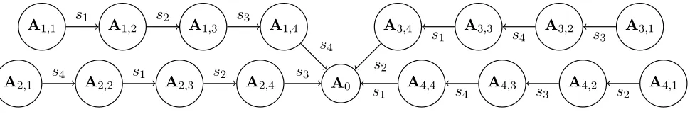
for a 4-partite protocol is depicted in Figure 1.
Of course, we must publish encodings that would allow the parties to choose their secrets and provide encodings for them. This means that together with the public parameters we also publish encodings of many plaintext elements {ti,` :i= 1, . . . , k, `= 1, . . . , N} (for a sufficiently
large N), for each ti,` we publish encoding of it relative to all the edges Ai0,i+i0−1 → Ai0,i+i0 for all i, i0 (index arithmetic modulo k+ 1). Party i then chooses random small coefficients ri,`
A0
A1,4
A1,3
A1,2
A1,1
A2,4
A2,3
A2,2
A2,1
A3,4 A3,3 A3,2 A3,1
A4,4 A4,3 A4,2 A4,1
s1 s2 s3
s4
s4 s1 s2 s3
s3
s4
s1
s2
s2
s3
s4
s1
Figure 1: Graph for a 4-partite key-agreement protocol.
of the encodings on that edge with the coefficient ri,`. We are now ready to describe our scheme N MKE = (KE.Setup,KE.Publish,KE.Keygen).
• KE.Setup(1λ, k): The setup algorithm takes as input the security parameter 1λ and the total number of playersk.
1. Run the parameter-generation and instance-generation of our graph-based encoding scheme for the graph consisting ofk chains with a common end-point, each of lengthk edges. Let
ei,j denote the j’th edge on the i’th chain.
2. Using the secret parameters, run the sampling procedure of the encoding scheme to choose random plaintext elements ti,` for i= 1, . . . , k and `= 1, . . . , N, and for each ti,` compute
also an encoding of it relative to all the edges ei0,j for j = i+i0 (mod k). Denote the encoding ofti,` on chain i0 (relative to edge ei0,i+i0modk) by Ci,`,i0.
The public parameters of the key-agreement protocol include the public parameters of the encoding scheme (i.e., the matrices for all the source nodesAi,1), and also the encoding matrices
Ci,`,i0 :i, i0 = 1, . . . , k, `= 1, . . . , N .
• KE.Publish(pp, i) : The i’th party chooses random small plaintext elements ri,` ← χ for ` =
1, . . . , N and then setsDi,i0 ←P
`Ci,`,i0·ri,` for alli0. It keepsDi,i as its secret and broadcast all the other Di,i0’s.
• KE.Keygen(pp, i,ski,{pubj}j6=i) : Party i collects all the matrices Di0,i (encoding the secrets
si0 relative to “its chain” i) and orders them according to j = i+i0. Namely, it sets Fj,i = Di+jmodk,i forj = 1, . . . k, then computes the productF∗i = (
Qk
j=1Fj,i)·Ai,1. Finally, partyi
applies the extraction procedure of the encoding scheme to obtain the secret key, settingssk=
Extract F∗i
.
Security. Unfortunately, we were not able to reduce the security of this candidate scheme to any “nicer” assumption. As such, at present the only evidence of security that we can offer is the failure of our attempts to cryptanalyze it.
The basic attack from Section 4.1 does not seem to apply here since the public parameters do not provide any encoding of zero (not even relative to A0). Similarly, the extended attacks do not
seem to apply since the only common end-point in the graph isA0, and no two paths that end at
A0 include an encoding of the same element.
Finally, we note that as for any other application of this encoding scheme, it seems that security would be enhanced by applying the additional safeguards that were discussed at the end of Section 3. That is, we can use Kilian-style randomization on the encoding side, by choosing k invertible matrices for each chain,Ri,1, . . . ,Ri,k, where the first and last are set to the identity and the others
are chosen at random. Then we can replacing each encoding matrixCin the public parameters by C0 :=R−1·C·R0 using the randomizer matrices R,R0 belonging to the two adjacent nodes. We
can also choose the first encoding matrix in each chain to have large entries.
This has no effect on the product of all the encoding matrices along the i0-th chain, but the new matricesC0 no longer have small entries, which seems to aid security. On the down side, this increases the size of the encodings roughly by a logq/lognfactor.
5.2 Candidate Branching-Program Obfuscation
We next describe how to adapt the branching-program obfuscation constructions from previous work [GGH+13a, BR14b, BGK+14, PST14] to use our encoding schemes. We remark that on some level this is the simplest type of constructions to adapt to our setting, since we essentially need only a single chain and there almost no issues of providing zero-encoding in the public parameters (or encodings of the same plaintext relative to different nodes in the graph).
Roughly speaking, previous works all followed a similar strategy for obfuscating branching programs. Starting from a given oblivious branching program, encoded as permutation matrices, they all applied Kilian’s randomization strategy to randomized these matrices, then added some extra randomization steps (mostly multiplication by random scalars) to protect against partial-evaluation and mixed-input attacks, and finally encoded the resulting matrices relative to specially-designed sets/levels. The specific details of the extra randomization steps are somewhat different between the previous schemes, but all these techniques have their counterparts in our setting. Below we explain how to adapt the randomization techniques from previous work to our setting, and then describe one specific BP-obfuscation candidate.
Matrices vs. individual elements. Our scheme natively encodes matrices, rather than individual elements. This has some advantages, for example we need not worry about attacks that mix and match encoded elements from different matrices. At the same time it also poses some challenges, in particular some of the prior schemes worked by comparing to zero one element of the resulting matrix at the end of evaluation, an operation which is not available in our case.
To be able to examine sub-matrices (or single elements), we adopt the “bookend encoding” trick from [GGH+13a]. That is, we add to our chain a new sourceu∗ and a new sinkv∗, with edges from u∗ to the old source and from the old sink to v∗. On the edge from u∗ we encode a matrix T which is only nonzero in the columns that we want to examine, and on the edge to v∗ we encode a matrixS which is only nonzero in the rows that we wish to examine. This way, we should have the matrix T·U·S encoded relative to a path u∗ ; v∗, and that matrix is only nonzero in the sub-matrix of interest. In the candidate below we somewhat improve on this by folding the source matrix Au∗ into the encoding of T, publishing instead the matrix Au∗·T (and in fact making T a single column vector).
that we multiply by both R and R−1 for each randomizer matrix R. One way to get randomizer matrices with bothR and R−1 small is using the facts that
I 0 R I −1 = I 0
−R I
, I R 0 I −1 =
I −R
0 I 0 I I R −1 = 0 I
I −R
, R I I 0 −1 =
−R I
I 0
.
Multiplying a sequence of these types of matrices above yields a high-entropy distribution of randomizer matrices with the desired property, and seemingly without obvious algebraic structure. Another family of matrices where both the matrix and its inverse are small are permutation matrices (and of course we can mix and match these families). Concretely, we speculate that a randomizer of the form
R= Π1·
0 I I R1
·Π2·
I 0
R2 I
·Π3·
R3 I
I 0
·Π4·
I R4
0 I
·Π5 (4)
(with the Πi’s random permutations and the Ri’s random small matrices) has sufficient entropy
and lack of algebraic structure to server as randomizers for our scheme.
We note that although these randomizers are far from uniform, there may still be hope of using some of the tools developed in [BR14b, BGK+14, PST14] (where the analysis includes a reduction
to Kilian’s information-theoretic argument). This is because the matrices before randomization are permutation matrices, and hence the random permutations Πi can be used to perfectly randomize
them. In this way, one can view the Ri’s are merely “safeguards” to protect against possible
weaknesses in the encoding scheme, and the Πi’s are “ideal model randomizers” than can be used
in an ideal-model analysis. So far we did not attempt such analysis, however.
Another way to introduce Kilian-type rerandomization in our setting is the aforementioned option of applying it “on the encoding side,” i.e., choosing random m×m invertible matrices P modulo q and setC0 ←P−1·C·P0.
Multiplicative binding and sraddling sets. Another difference between our setting and that of GGH or CLT is that the previous schemes support encoding relative to arbitrary subsets of a universe set, so there are exponentially many potential sets to use. In our scheme the encoding is relative to edges of a given graph, and there can be only polynomial many of them. This difference seems particularly critical in the design of sraddling sets [BGK+14, PST14].
On a second look, however, this issue is more a question of modeling, rather than a real difference. The different encoding sets in the “asymmetric variants” of [GGH13b, CLT13] are obtained just by multiplying by different random secret constants (e.g., the zi’s from GGH), and
we can similarly multiply our encoding matrices by such random constants modq (especially when working over a large polynomial ring). We use that option in the candidate scheme that we describe below.
5.2.1 A Concrete BP-Obfuscation Candidate
For our concrete candidate below we work over a large polynomial ring of dimensionk, and we will use small-dimension matrices over this ring (roughly as high as the dimension of the underlying branching program).
LetSym(w) be the set ofw×wpermutation matrices and consider a length-nbranching program over`bit inputs:
BP={(ind(i),Bi,0,Bi,1 :i∈[n],ind(i)∈[`],Bi,b ∈Sym(w)}
For a bit position j ∈ [`], let Ij be the steps in the branching program that examines j’th input
bit: Ij ={i∈[n] :ind(i) =j}. We obfuscateBP as follows:
• Following the original construction of [GGH+13c] we embed theBi,σ’s inside higher-dimension
matrices with random elements on the diagonal, but in our case it is sufficient to have only two such random entries (so the dimension only grows form w to w+ 2). Denote the higher-dimension matrices by B0i,σ.
We also follow the original construction of [GGH+13c] by applying the same transformation to a “dummy program”DPof the same length that consists of only the identity matrices, letD0i,σ be the higher-dimension dummy matrices.
• We proceed to randomize these branching programs a-la-Kilian “on the plaintext side,” by choosing randomizing matricesRi’s as per the form of Eqn. (4) such that bothRi andR−i 1 are
small, and setting B00i,σ =Ri−1B0i,σR−i1. The dummy program is randomized similarly.
• We then prepare (w+ 2)×(w+ 2) “bookend matrices” S,S0, and “bookend column vectors” t,t0. S is random and small except the first row which is zero, t is random and small except the second entry which is zero, and similarly for S0 and t0, subject toS0·t0 = S·t. Then we set ˜S=SR−01 and ˜t=Rnt, and similarly ˜S0 =S0R−01 and ˜t0 =Rnt0.
• We also sample random small scalars {αi,0, αi,1, αi,00 , α0i,1 : i ∈ [n]}, subject to constraint:
Q
i∈Ijαi,0 =
Q
i∈Ijα 0 i,0 and
Q
i∈Ijαi,1 =
Q
i∈Ijα 0
i,1. These are used for the “plaintext-side”
multiplicative bundling.
We set B∗i,σ =B00i,σ·αi,σ for the main program and similarly D∗i,σ =D00i,σ·α0i,σ for the dummy
program.
• Next we use our encoding scheme to encode these matrices relative to a graph with two chains with a common end-point, each of length n+ 2. Namely we have A1 → . . . → An+2 and
A01 →. . .→A0n+1 →An+2.
For eachi∈[n], we encode the two matrices B∗n−i+1,b relative to the edge Ai →Ai+1, i.e., we
have
Cn−i+1,b·Ai =Ai+1·B∗n−i+1,b+Ei,b
for some small error Ei,b. Similarly we encode the dummy program with the two matrices
D∗n−i+1,b encoded relative to the edge A0i→A0i+1, i.e.,
• Encode ˜S,S˜0 relative to the edges leading to the common sink, i.e. compute the encoding
matricesCS,C0S0 such that
CS·An+1 =An+2·S˜+ES and CS00·A0n+1 =An+2·S˜0+E0S0
• Compute the encoded bookend vectors, folded into the two sources A1 and A01, namely a =
A1·˜t+et and a0=A01·t˜0+e0t.
• We next apply both the multiplicative bundling and the the Kilian-style randomizationalso on the encoding side. Namely we sample random full-rank matricesP0, . . . ,PnandP00, . . . ,P0n, and
also random scalars moduloq {βi,0, βi,1, βi,00 , βi,10 :i∈[n]}, subject to constraints
Q
i∈Ijβi,0 =
Q
i∈Ijβ 0 i,0 =
Q
i∈Ijβi,1 =
Q
i∈Ijβ 0 i,1 = 1.
We then set ˆCi,σ =P−i−11·Ci,σ·Pi·βi,σ and ˆC0i,σ =P0−i−11·C0i,σ·P0i·βi,σ0 , and also ˆCS =CS·P0
and ˆC0
S0 =C0
S0 ·P00 and ˆa=Pn−1a and ˆa0=P0−n1a0.
• The obfuscation consists of all the matrices and vectors above, namely
O(BP) =
ˆ CS,
ˆ
Ci,σ :i∈[n], σ∈ {0,1} ,aˆ
,
ˆ C0
S0,Cˆ0i,σ :i∈[n], σ∈ {0,1} ,aˆ0
Evaluation. On inputx∈ {0,1}` the user choose the appropriate encoding matrices ˆC
i,0 or ˆCi,1
depending on the relevant input bit (and the same for ˆC0i,0 or ˆC0i,1) and then multiply in order
setting
y = CˆS·( n
Y
i=1
ˆ
Ci,x[ind(i)])·a = An+2· S·( n
Y
i=1
B00i,x[ind(i)])·t
+e
and
y0 = Cˆ0 S0 ·(
n
Y
i=1
ˆ C0
i,x[ind(i)])·a0 = An+2· S0·( n
Y
i=1
D00i,x[ind(i)])·t0+e0,
The output is 1 if ky−y0k< q3/4 and 0 otherwise. Note that indeed if Qn
i=1Di,x[ind(i)] =I then
both yand y0 are roughly equal toAn+2·S·t·(Qni=1αi,x[ind(i)]), as needed.
Security. As before, this is merely a candidate and we do not know how to reduce its security to any “nice” assumption. However the type of attacks that we know against these scheme do not seem to apply to this candidate.
References
[Ajt99] Mikl´os Ajtai. Generating hard instances of the short basis problem. InICALP, pages 1–9, 1999.
[AR13] Divesh Aggarwal and Oded Regev. A note on discrete gaussian combinations of lattice vectors. CoRR, abs/1308.2405, 2013.
[BF01] Dan Boneh and Matthew K. Franklin. Identity-based encryption from the Weil pairing. In CRYPTO, pages 213–229, 2001.
[BF03] Dan Boneh and Matt Franklin. Identity-based encryption from the Weil pairing. SIAM J. of Computing, 32(3):586–615, 2003. extended abstract in Crypto’01.
[BGG+14] Dan Boneh, Craig Gentry, Sergey Gorbunov, Shai Halevi, Valeria Nikolaenko,
Gil Segev, Vinod Vaikuntanathan, and Dhinakaran Vinayagamurthy. Fully
key-homomorphic encryption, arithmetic circuit abe and compact garbled circuits.
In PhongQ. Nguyen and Elisabeth Oswald, editors, Advances in Cryptology
EUROCRYPT 2014, volume 8441 of Lecture Notes in Computer Science, pages 533– 556. Springer Berlin Heidelberg, 2014.
[BGK+14] Boaz Barak, Sanjam Garg, Yael Tauman Kalai, Omer Paneth, and Amit Sahai.
Protecting obfuscation against algebraic attacks. In PhongQ. Nguyen and Elisabeth Oswald, editors,Advances in Cryptology EUROCRYPT 2014, volume 8441 ofLecture Notes in Computer Science, pages 221–238. Springer Berlin Heidelberg, 2014.
[BGW05] Dan Boneh, Craig Gentry, and Brent Waters. Collusion resistant broadcast encryption with short ciphertexts and private keys. In Victor Shoup, editor, Advances in Cryptology CRYPTO 2005, volume 3621 ofLecture Notes in Computer Science, pages 258–275. Springer Berlin Heidelberg, 2005.
[BR14a] Zvika Brakerski and Guy N. Rothblum. Virtual black-box obfuscation for all circuits via generic graded encoding. In Yehuda Lindell, editor, TCC, volume 8349 of Lecture Notes in Computer Science, pages 1–25. Springer, 2014.
[BR14b] Zvika Brakerski and GuyN. Rothblum. Virtual black-box obfuscation for all circuits via generic graded encoding. In Yehuda Lindell, editor, Theory of Cryptography, volume 8349 of Lecture Notes in Computer Science, pages 1–25. Springer Berlin Heidelberg, 2014.
[BS03] Dan Boneh and Alice Silverberg. Applications of multilinear forms to cryptography. Contemporary Mathematics, 324:71–90, 2003.
[BZ14] Dan Boneh and Mark Zhandry. Multiparty key exchange, efficient traitor tracing, and more from indistinguishability obfuscation. In Juan Garay and Rosario Gennaro, editors, Advances in Cryptology CRYPTO 2014, volume 8616 of Lecture Notes in Computer Science, pages 480–499. Springer Berlin Heidelberg, 2014.