Optical Fibre Bragg Grating Analysis Through FEA and its Application to Pressure Sensing

(1)

OPTICAL FIBRE BRAGG GRATING

ANALYSIS THROUGH FEA AND ITS

APPLICATION TO PRESSURE

SENSING

NITHILA DEDIYAGALA

A thesis submitted in fulfilment of the requirements for the degree of

DOCTOR OF PHILOSOPHY

2019

COLLEGE OF ENGINEERING AND SCIENCE

(2)

II

DECLARATION

“I, Nithila Dediyagala, declare that the PhD thesis entitled ‘Optical fibre Bragg grating analysis through FEA and its application to pressure sensing’ is no more than 100,000 words in length including quotes and exclusive of tables, figures, appendices, bibliography, references and footnotes. This thesis contains no material that has been submitted previously, in whole or in part, for the award of any other academic degree or diploma. Except where otherwise indicated, this thesis is my own work”.

(3)

III

ABSTRACT

The focus of this thesis is developing optical fibre Bragg grating (FBG) pressure sensors with enhanced sensitivity for use in a low (gauge) pressure range (0 - 50 kPa) together with understanding observed non-linear behaviour. To appreciate the behaviour of FBG sensor spectra, it is necessary to understand geometrical and material properties of FBGs. The thesis is an in-depth investigation of the behaviour of FBGs including their manufacturing and fabrication process details. A new computational approach has been introduced to simulate FBG structures based on how the FBG fabrication process produces changes in refractive index.

(4)

IV

computational tool which will be useful in further research to understand the behaviour of a variety of FBG structures. For this study, material properties of standard single mode fibre (SMF-28) was considered. However, the model is able to simulate any optical fibre used in FBG fabrication by changing the material properties.

The thesis also considers the understanding of FBG pressure sensors and observed non-linear behaviour. Therefore, a thorough literature review was carried out to find the influence of structural and material properties of optical fibres and FBGs which is believed to be the cause of non-linear behaviour. It investigates in depth the birefringence effect on fibres due to point load and distributed load on FBGs using the Structural Mechanics and Wave Optics module in COMSOL software. Many research studies have employed a plane strain assumption for structural mechanics problems; however, they do not clearly explain the true nature of FBGs under stress generalized strain. This study overcomes that problem by introducing proper mathematical equations to develop 3-D behaviour in a 2-D computational model. The behaviour of a distributed load on FBGs was discussed in detail with the help of the computational model. It provides new information about an asymmetric peak produced as a result of birefringence effects.

(5)

V

LIST OF PUBLICATIONS

Peer reviewed conference papers:

Dediyagala, N., Baxter, G. W., Sidiroglou, F. & Collins, S. F. 2016, FEA and FFT modelling of harmonics from fibre Bragg gratings, paper presented at the 2016

Australian Institute of Physics (AIP) Congress, Brisbane, Australia.

Dediyagala, N., Baxter, G. W., Sidiroglou, F. & Collins, S. F. 2014, Comparison of experimental, theoretical and Finite Element Analysis on fibre Bragg grating

pressure sensitivity, paper presented at the 2014 Australian Institute of Physics

(6)

VI

ACKNOWLEDGEMENTS

My journey through PhD in Victoria University has given me a transition period of my life. Completion of the thesis is the end of that journey and one of my biggest achievements. This journey would not be completed without tremendous support given to me by many great people around me. Hence, it is my duty to thank and acknowledge all of them and share all the credit with them.

First and foremost, I would like to dedicate my sincere thanks to Professor Gregory Baxter for his continued support, guidance and valuable comments as my senior supervisor. I would like to dedicate my heartfelt appreciation for my co-supervisor, Professor Stephen Collins, for his great guidance, valuable and constructive comments. This thesis would not be completed without his tremendous support throughout the entire process. My sincere thanks go to co-supervisor, Dr. Fotios Sidiroglou for his constructive suggestions and encouragements during this whole time. I greatly appreciate their kindness and friendship during the research. Thanks also go to Dr. Nicoleta Dragomir for her valuable suggestions and comments in the early stage of the research.

I am deeply grateful for Victoria University for accepting me as a PhD student and providing financial support for the proposed project. I would also like to thank all administration staff and technical staff in the School of Engineering and Science for their valuable support during this period. This is also the time to remind the support and encouragement from dear colleagues Dr. Robab Antonios, and Dr. Wan Hafiza, who have become forever friends of mine. I am also indebted to the support provided by team of COMSOL Multiphysics® simulation software. This project would not be possible and successful without their useful comments and support.

(7)

VII

in law, Mallika Dias, for her continuous support and inspiration throughout my research.

(8)

VIII

LIST OF FIGURES

Figure 1.1: Patent data accepted in (Patent Insight Pro, 2011) shows the differentiation in terms of number of patent issued of distributed sensing approaches, Bragg grating and interferometric sensors (Kersey, 2012) ... 1

Figure 1.2: Fibre Optic Sensor Global Consumption Market Forecast (Values in $ Billions) (Electronicast, 2012) ... 2

Figure 2.1: Schematic diagram of (a) end view and (b) side view of an optical fibre - x, y and z show the direction of axis of the fibre which is used throughout the study ... 9

Figure 2.2: Schematic diagram of transmission of a light ray in an optical fibre 10

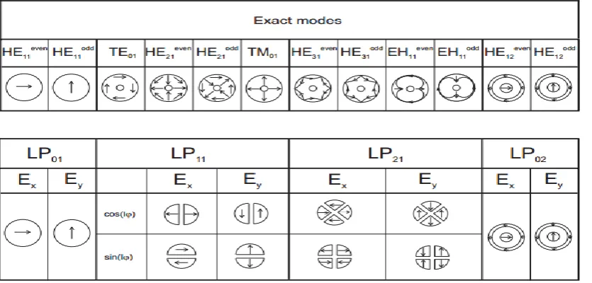
Figure 2.3: Electric field of lowest 12 modes of corresponding LP modes in step index fibre (Ma, 2009). ... 12

Figure 2.4: Normalized frequency (V) Vs normalized propagation constant (b) (Keck, 1981). The vertical line applies to (⅔)λB for SMF-28 fibre (assuming λB

=1550 nm). ... 13

Figure 2.5: Transmission and reflection spectra due to FBG... 20

Figure 2.6: Optical system for interferometric inscription of FBGs (a) transverse holographic method and (b) phase mask method ... 22

Figure 2.7: Optical system for Interference Lithographic method ... 23

Figure 2.8: Image of 400 nm grating in photoresist Transfer the photoresist grating pattern into substrate (fused silica) - (Chen & Schattenburg, 2004) ... 25

Figure 2.9: Image of Scanning Electron Microscopy of 400 nm grating in fused silica (Buchwald, 2007) ... 25

(13)

XIII

Figure 2.11: The induced index changes along the longitudinal axis of fibre core to a FBG - the colour spectrum shows variation of index change in FBG region

... 27

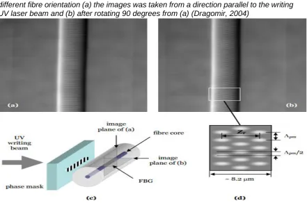
Figure 2.12: DIC images of the fibre core containing Bragg grating, recorded for two different fibre orientation (a) the images was taken from a direction parallel to the writing UV laser beam and (b) after rotating 90 degrees from (a) (Dragomir, 2004) ... 28

Figure 2.13: DIC microscopy images of FBG in core region of Type 1 fibre at different orientation to the writing beam (a) Images of fibre orientation is perpendicular to the writing beam (b) Images of fibre orientation is parallel to the writing beam (c) schematic diagram of writing technique and image planes orientation to the writing beam (d) Schematic diagram of (b) showing the interleaving planes belongs to index modulation of Ʌpm and Ʌpm/2; ZT is Talbot length (Rollinson, 2012) ... 28

Figure 2.14: Modelled intensity variation in the core area of the fibre due to contribution of multiple diffraction orders from phase mask fabrication (Kouskousis et al., 2013) ... 29

Figure 2.15: Reflection (a) and transmission (b) of uniform Bragg grating ... 32

Figure 3.1: Schematic diagram of typical FBG sensing system... 42

Figure 4.1: Representation of Boundary Value Problem ... 48

Figure 4.2: Schematic diagram of volume discretization method in FEA (a) the object which represent the problem (b) the object is divided into number of small units which is called elements (c) elements are a combination of points and lines or surfaces... 50

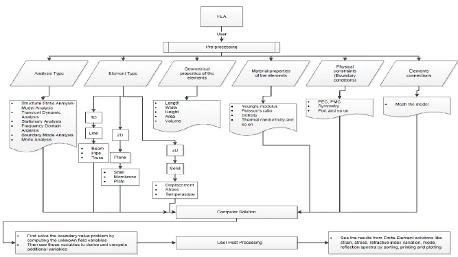
Figure 4.3: Flow chart of FEA process ... 51

Figure 4.4: End face of optical fibre of SMF-28 and its mesh diagram ... 53

(14)

XIV

Figure 4.6: (a) Electric field variation of HE11 in the fibre surface and (b) Intensity

variation along z direction across fibre core (b) at λB ... 55

Figure 4.7: (a) Electric field variation of HE11 in the fibre surface and (b) intensity

variation along z direction across fibre core at 2λB ... 55

Figure 4.8: Electric field variation of HE11 in the fibre surface and electric field

variation along x direction across fibre core at (⅔)λB ... 56

Figure 4.9: Electric field variation of TM01 in the fibre surface and electric field

Figure 4.10: Electric field variation of TE01 in the fibre surface and electric field

Figure 4.11: Electric field variation of HE21 in the fibre surface and electric field

Figure 4.12: Electric field variation of each mode in the fibre surface x direction across the fibre core at (⅔)λB ... 58

Figure 4.13: Schematic diagram of phase mask structure ... 59

Figure 4.14: Schematic diagram of beam splitting at phase mask with respect to the angle of incident ... 60

Figure 4.15: Schematic diagram of FBG writing process using phase mask method for a unit cell ... 62

Figure 4.16: Schematic diagram of boundary conditions on the model, inside of dashed line will be used to show the relevant mesh in Figure 4.18 ... 65

Figure 4.17: Schematic diagram of S-parameter ... 67

Figure 4.18: Mesh diagram of the FEA domain around phase change area in Figure 4.16 ... 68

(15)

XV

Figure 4.20: Diagram of boundary conditions for light propagation through a FBG ... 71

Figure 4.21: Mesh diagram of optical fibre ... 72

Figure 4.22: Simulated intensity spectrum along the fibre core using phase mask method (red and yellow lines represent the line scans along the fibre core and Talbot length respectively)... 73

Figure 4.23: Line profile of intensity distribution at -71.00 µm along the fibre core ... 74

Figure 4.24: Evaluated harmonics using FFT for intensity distribution of Figure 4.23, i.e. line scan at -71.00 µm ... 74

Figure 4.26: Evaluated harmonics using FFT for intensity distribution of Figure 4.25 i.e. line scan at -71.75 µm ... 75

Figure 4.28: Evaluated harmonics using FFT for intensity distribution of Figure 4.27, i.e. line scan at -73.35 µm ... 76

Figure 4.29: FBG pattern was obtained using phase mask technique, the colour line represents the refractive index value of FBG pattern ... 79

Figure 4.30: Simulated FBG reflection spectrum at λB for complex FBG pattern of

Figure 4.29, obtained by phase mask method... 80

Figure 4.31: Simulated FBG reflection spectrum at 2λB, obtained for complex FBG

pattern ... 81

Figure 4.32: Resultant FBG reflection spectrum at (⅔)λB by complex FBG pattern

... 82

(16)

XVI

Figure 5.1: Possible forms of pressure exertion on an optical fibre (a) Transverse compressive load, (b) Tensile and compressive strain, (c) Uniform pressure .. 87

Figure 5.2: Schematic diagram of 2D cross section of point load (a) and distributed load (b) on FBG ... 88

Figure 5.3: Schematic diagram of a 3-D cylindrical fibre (a) and simplified (2-D cross section) view of the same FBG due to axial symmetry (b) ... 88

Figure 5.4: Schematic diagram of computational domain for point load (a) and mesh diagram (b) ... 93

Figure 5.5: Schematic diagram of computational domain for distributed load on an optical fibre (a) and boundary conditions (b) ... 94

Figure 5.6: Schematic diagrams of bare fibre (a) and polymer coated fibre (b) experiencing uniform pressure in cylindrical coordinates ... 94

Figure 5.7: Screen shot of wave equation is set under electromagnetic wave, frequency domain in COMSOL ... 96

Figure 5.8: The domains of distributed load with its defining mesh ... 97

Figure 5.9: Mesh diagram on the uniform pressure sensing on bare fibre ... 98

Figure 5.10: Effective mode index variations, with and without stress-optic relations when reference temperature is 20 0_{C (a) and 1000}0_{C (b) ... 99}

Figure 5.11: Effective mode variation with plain strain and generalized plain strain when reference temperature is 1000 0_{C ... 100}

Figure 5.12: Power flow across modes across end face of the fibre. ... 101

Figure 5.13: Power flow variation on the end face of the fibre due to 0 N (a), 20 N (b) and 40 N (c) ... 102

Figure 5.14: Stress variations along x (a), y (b) and z direction (c) and along the middle of the fibre as shown in red line (d) ... 103

(17)

XVII

Figure 5.16: Graph of effective mode index variations with applied load for distributed load fibre ... 105

Figure 5.17: Intensity variation on the end face of the fibre with different loads ... 106

Figure 5.18: Intensity of all effective mode values along z direction ... 106

Figure 5.19: Stress variations along x (a), y (b), z direction (c) along middle of the fibre as shown in red line (e) and relevant effective mode index for different loads (d) ... 107

Figure 5.20: Stress variations along x (a), y (b), z direction (c), along middle of the fibre as shown in red line (d) and, relevant effective mode index for different loads ... 108

Figure 5.21: Index of refraction changes in (a) x and y directions are calculated using equations and simulation results (b) birefringence, in the centre of the fibre ... 109

Figure 5.22: (a) Bragg wavelength change in x and y directions and (b) Bragg wavelength in x and y directions for a distributed load ... 110

Figure 5.23: Graph of radial axial and radial strain (a) and stress (b) vs pressure ... 110

Figure 5.24: Pressure vs wavelength shift ... 111

Figure 5.25: (a) Wavelength shift Vs pressure and (b) 2D cross section view of structure deformation due to pressure experience (b) ... 112

Figure 5.26: Strain (a) and stress (b) variation along axial and radial directions on the centre of the fibre ... 113

(18)

XVIII

Figure 5.28: Wavelength shift vs pressure, without any diameter deduction of the fibre cladding (a), wavelength shift after 30 µm deduction from the cladding of the fibre ... 115

(19)

XIX

LIST OF TABLES

Table 1.1: Collection of exemplary standards for medical pressure analysis .... 7

Table 1.2: Medical areas and the research impact on FBG based sensors ... 8

Table 2.1: Properties of SMF-28 fibre ... 13

Table 2.2: Physical and material properties of SMF-28 (FEA simulation) ... 14

Table 2.3: Types of FBGs, their characteristics and properties ((Canning, 2008)) ... 18

Table 3.1: Summary of FBG-based pressure sensors, in order of pressure sensitivity for bare/polymer coated/mechanical/force multipliers ... 36

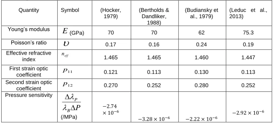
Table 3.2: Reported material values for the silica fibre and the calculated pressure sensitivity ... 42

Table 4.1: Parameters and values for the simulation* ... 59

Table 4.2: The calculated and defined parameters for the simulation ... 66

Table 4.3: Results of spectral components of SMF-28 for simulated FBG patterns: evaluated grating periods using FFT analysis and their harmonics, fraction of period compare to the phase mask period, calculated wavelength using Equation 2.10 and ratio of calculated wavelength to Bragg wavelength ... 77

Table 4.4: Results of diffracted efficiency of harmonics for different line scans and the expected efficiencies according to the manufacturer information ... 77

Table 4.5: Calculated Talbot length (in free space) of the diffracted pattern produced by the phase mask with period of 1.066 µm, index of refraction of 1.488 and wavelength at 244 nm. ... 78

Table 5.1: Material properties of selected polymers ... 112

Table 5.2: Material properties of PTEF and PDMS ... 114

(20)

XX

Table 5.4: Pressure sensitivity by different materials under different pressure and changing diameter ... 116

(21)

1

CHAPTER 1:

Introduction

1.1 OVERVIEW

The invention of fibre optic wire or “Optical Waveguide Fibres” by Corning Glass researchers in 1960 has had a tremendous impact on global communication as it revolutionized the telecommunications industry. Fibre optics is a major industry and today it plays a key role in modern day life such as long-distance telephone service, internet and use in health care services. The invention of the fibre-optic gyroscope in 1976 led fibre optic sensor explorations for the next ten years (McLandrich & Rast, 1978). Commercialization of optical fibres provides more components for other uses which have led to the opportunity for their use as sensors in many field applications. Since then various ideas have been suggested and techniques have been developed for many measurands and applications. According to statistics presented at OFS-15 (Optical Fibre Sensors Conference held in Portland, Oregon, USA 2002), strain and temperature are the most highly studied measurands, with fibre Bragg grating (FBG) sensors becoming increasingly popular. According to statistics of OFS-22, FBG sensors had the highest number of patent issued among optical fibre sensors (Kersey, 2012). Figure 1.1 illustrates FBG sensor popularity, as derived from an industry survey (Patent Insight Pro, 2011).

(22)

2

FBG sensors have attracted a considerable amount of interest in a vast range of applications due to their wavelength-encoded character and linear response to changes in various measurands (Hill & Meltz, 1997; Othonos & Kyriacos, 1999). Figure 1.2 shows the annual investment in fibre optics sensors including FBG sensors from 2011 - 2016. It shows 20.5% (from $1.34 to $3.39 billion) of estimated annual growth rate of fibre optics sensors, which further signifies their importance (Electronicast, 2012; Méndez, 2007).

Figure 1.2: Fibre Optic Sensor Global Consumption Market Forecast (Values in $ Billions) (Electronicast, 2012)

1.2 WHY OPTICAL FIBRE TECHNOLOGY? (OPTICAL BASED METHOD

AND ADVANTAGES)

(23)

3

chemical, biological, aviation, healthcare, automation industries, illustrating how it has been valuable and a promising technology for industrial applications (Annamdas, 2012).

Fibre optic sensors can be categorized into extrinsic and intrinsic sensors (Othonos & Kyriacos, 1999). Extrinsic sensors are mostly used in harsh condition where most of the other sensors are unable to operate. In these sensors, fibre is used as an information carrier but the interaction between the light and the quantity of the measurement takes place outside of the fibre itself. This means the transducer is external to the fibre; hence, these sensors are called extrinsic sensors. They are mostly used in industry to measure rotation, vibration velocity, displacement, twisting, torque and acceleration. In contrast, intrinsic sensors behave differently where the optical fibre becomes the sensing element itself by keeping the propagating light inside and which experiences modulation when the fibre is subjected to pressure, strain or temperature variation. These sensors are used to measure intensity, phase, polarization, wavelength or transit time of light. The simplicity of intrinsic sensors has attracted many industries like, aviation, civil engineering for physical measurements.

Currently available fibre optic sensors can be mainly classified into four major categories based on the operating principle:

1. Intensity

2. Phase (interferometric) 3. Polarization

4. Wavelength

Their advantages and disadvantages for pressure sensing are discussed below.

(24)

4

visibility). The next sensor type are polarization-modulated fibre optics sensors, which were not successful in pressure sensing in hazardous conditions due to its bulk size. Hence, all three sensor types have been limited in commercial use due to the issues above. However, the fourth sensor type, namely FBG sensors which are based on wavelength/spectrum modulation have been attractive to many industries due to their ability to overcome the aforementioned issues and offer specific advantages. FBG sensors and their advantages will be discussed below.

1.3 WHY FIBRE BRAGG GRATING (FBG) PRESSURE SENSORS?

Pressure measurement is vital in many industrial applications: aviation, bio-medical, oil and gas are some of them. Many sensors have been commercialized for pressure measurements from extreme vacuum (10-12_{Pa) to explosion (10}+12

Pa), the latter implying a flammable or harsh environment in some fields of application. In this range, optical fibre sensors have been identified as a potential solution for use as pressure sensors (Pinet, 2011) due to properties which are outlined in section 1.2.

Optical fibre photosensitivity was first discovered in germanium-doped silica optical fibres when an optical fibre core was exposed to a periodic pattern of ultraviolet (UV) light by Hill and co-workers (Hill, 2000; Hill et al., 1993). During the exposure to UV light, there was some intensity of light back-reflected which increased with time. Spectral responses confirmed the reflectivity was a result of a periodic modulation of the photo-induced refractive index change created along the core of the optical fibre. This triggered a new class of in-fibre component, now known as a Fibre Bragg Grating (FBG). The resultant central wavelength of back reflected light of a FBG depends on the effective index of refraction of the core and the grating periodicity. When a FBG experiences strain or a temperature change the effective index of refraction and grating periodicity are also affected. As a result, the changes of these two physical parameters have provided a means to measure temperature and strain variations. FBGs have hence emerged as a favourable sensing element owing to their potential use in measuring strain, temperature and pressure.

(25)

5

compression and impact, its material and physical properties change such as refractive index and grating length, with the Bragg condition providing the reflection wavelength of light launched into the fibre. Therefore, FBGs have become more popular in pressure, strain and temperature measurement. Their versatility, reliability and ease of embedding in a variety of structures make their use possible in smart structure applications. Moreover, the size of these sensors has been carefully considered and developed for biomedical application. FBGs are also popular in applications like robotics due to resolution, sensitivity and dielectric properties and multiplexing capability.

FBG sensors are popular not only for one parameter sensing but also multi- parameter sensing such as strain and temperature. Many sensors have been reported for multi-parameter sensing such as strain and temperature measurement simultaneously using pairs of FBGs operating at two different wavelengths (Brady et al., 1997; Echevarria et al., 2001) or using two different types of FBGs (Shu et al., 2002). A multi-axis strain sensor has been reported for multidimensional strain measurement such as transverse and longitudinal strain sensing using FBGs inscribed in birefringent optical fibre (Udd et al., 2002; Udd et al., 2000)

(26)

6

Although FBGs are potential candidates for pressure sensors, some drawbacks have been identified. FBGs inscribed in bare silica fibre exhibit a linear response over a large pressure range (0-70 MPa) but their sensitivity is low due to their material properties (Othonos & Kyriacos, 1999). Fibre is made of glass, which is less stiff than metal but stiffer than plastics, having a high Young’s modulus and low Poisson’s ratio. Although the pressure response is linear at high pressures, at moderate pressure (< 0.2 MPa) it is difficult to measure due to the very low sensitivity (Hill & Meltz, 1997). Furthermore, the response has been observed to become non-linear (Bal et al., 2011; Lawrence et al., 1999). Modification of the physical properties of optical fibre by application of a suitable coating has been pursued by many authors, including for improving their response to external pressure, as noted by Giallorenzi et al. (1982). Thus, having considered the above issues, the main objective in this research is to investigate the behaviour of FBGs at moderate (gauge) pressures (0 – 0.5 atm, i.e. 0 - 50 kPa) when an optical fibre is coated with a polymer material, since this should improve their pressure response, by lowering the Young’s modulus and increasing their Poisson’s ratio. This will include studies of various polymer materials as fibre coatings and noting how this affects the sensitivity of FBG pressure sensitivity in each case.

1.4 MOTIVATION AND SIGNIFICANCE

(27)

7

spectra, their behavior under pressure and the effect of coating materials. Therefore, the main objectives of the study can be stated as follows:

• Model FBGs structures and their spectra using Finite Element Analysis (FEA) methods

⎯ Analyze their spectra for better understanding of their relationship with the underlying FBG complex refractive index variation;

• Model FBGs with different polymer coatings using a FEA method to identify suitable materials for enhancing the pressure sensitivity at moderate pressures ⎯ Compare the results with existing literature to confirm efficacy of the findings

in simulations.

As an example, Table 1.1, shows that for the medical fields of urology, neurology, gastroenterology and ophthalmology, the pressure range of interest is between 0 – 30 kPa. Therefore, the pressure range under consideration (0 - 50 kPa) is highly applicable in these fields.

Table 1.1: Collection of exemplary standards for medical pressure analysis (Poeggel et al., 2015)

(28)

8

pressure range of 0 – 50 kPa is of interest. There are a limited number of publications that have been published in the areas listed in Table 1.2, showing the potential for the sensor investigated in this study using computational design. Consequently, there is significant motivation to explore the feasibility of developing a FBG pressure sensor for the 0 – 50 kPa range. This thesis achieves that objective by developing a COMSOL model to test the effectiveness of using a polymer coating on a standard glass fibre with an embedded FBG.

(29)

9

CHAPTER 2:

Optical Fibres, FBGs and FBG fabrication

2.1 OVERVIEW

This chapter focuses on optical fibres, their operational characteristics including waveguide modes related to different wavelengths. It also provides a detailed insight into light propagation through optical fibres and the resultant number of waveguide modes. It deeply discusses fibre Bragg gratings (FBGs), their classification, fabrication methods and the theory of their operation including their spectra.

2.2 OPTICAL FIBRE AND ITS PROPERTIES

An optical fibre is a light guiding structure which enables light to propagate from one end to the other end of the structure. The phenomenon of light propagation occurs due to its material and geometrical properties. An optical fibre’s geometrical representation with cylindrical shape of layers is shown in Figure 2.1. These cylindrical layers are made of either glass or plastic material which has different dielectric properties that allow light propagation.

(a) (b)

Figure 2.1: Schematic diagram of (a) end view and (b) side view of an optical fibre - x,

y and z show the direction of axis of the fibre which is used throughout the study

The centre of an optical fibre is called the core and has higher refractive index ( 𝑛₁) than the cladding layer ( 𝑛₂). As a result, light is confined in the core area of the structure. When a light beam is incident on the fibre–air interface with

x y

z y

(𝑛₁)

y

x

y

(30)

10

an angle θ, as shown in Figure 2.2, it propagates through the structure as it experiences total internal reflection at the core-cladding interface.

Figure 2.2: Schematic diagram of transmission of a light ray in an optical fibre

At the core-cladding interface the critical angle (𝜑𝑐) is given by Equation 2.1.

sin φ_c=n2 n1

Equation 2.1

The amount of light propagating through the structure depends on the light beam characteristics at the air-fibre interface, as not all rays will be coupled into a guided mode of the optical fibre. Therefore, it is necessary to determine the Numerical Aperture (NA), which measures the light gathering capacity.

At an air-fibre interface, if there is no surface irregularity and surface roughness, the NA is determined by the refractive indices difference between core and cladding areas, where the maximum value of sinθ for a ray to be guided, corresponding toφ_c, is given by the following equation:

sin 𝜃_𝑚𝑎𝑥=NA=√n₁2_-n 2

2 Equation 2.2

The coupling efficiency of launching light into propagating modes in the fibre depends on the NA; the smaller the NA the smaller the acceptance angle. Hence, coupling with a small NA requires careful consideration of optical components and precise mechanical positioning and alignment of the optical fibre. In contrast, a larger NA has a larger acceptance angle which can be easily aligned with the fibre and it is more effective in light gathering. However, in situations where the incident angle is larger than arsin (NA), the light is not guided through the core

(31)

11

properly and the loss of light will be high. This can be reduced by using lenses to ensure the light beam is directed into the acceptance cone of the fibre.

The transmission of light along the optical fibre can be explained by a set of Maxwell’s equations in electromagnetic theory. These describe the behaviour of optical fibre including its properties such as absorption, attenuation and dispersion. The behaviour of a transmitted wave is described by modes which represent the distinct waveform transmitted through the fibre according to its geometrical structure, material properties and existing boundary conditions. Fibre modes can be categorized into two types: radiation modes and guided modes. Radiation modes carry energy out of the core and disappear while the guided modes carry energy and information along the fibre. The guided modes have particular mode profiles due to their electric (E) and magnetic (H) field configuration during the light propagation. Generally, there are two types of modes existing in planar and cylindrical waveguides. They are TE and TM modes, where E and H are zero along the propagation direction. In addition to those modes in cylindrical waveguides, hybrid modes (where E and H are non-zero in the direction of propagation) occur as a result of skew ray propagation. In telecommunication-grade optical fibres, the relative refractive index difference

𝛥 ~ 0.003, with

𝛥 =𝑛1− 𝑛2 𝑛₁

Equation 2.3

Therefore, it satisfies the weak guidance approximation where the relative refractive index difference 𝛥 ≪ 1 (Gloge, 1971). Under the weak guidance condition, longitudinal fields are very small compared to transverse components. Therefore, it is assumed that the fibre modes are transverse and linearly polarized in one direction, which is called a linearly polarized (𝐿𝑃𝑙𝑚) mode. The optical

properties of 𝐿𝑃_𝑙𝑚 modes (Gloge, 1971) and its propagation constant can be obtained by solving eigenvalue equations (Snyder & Love, 2012). Figure 2.3 shows the electric field intensity profile with their electric field profile of the lowest four 𝐿𝑃_𝑙𝑚 modes (Ma, 2009; Poole et al., 1994).

(32)

12

Figure 2.3: Electric field of lowest 12 modes of corresponding LP modes in step index fibre (Ma, 2009).

Depending on the number of modes guided through a particular fibre, it can be categorized into single mode or multimode. Single mode fibre supports one guided mode (𝐻𝐸11) whilst multimode has more than one mode. The number of

modes guided through the structure depends on the operating wavelength (𝜆), radius of the core (𝑎) and numerical aperture (𝑁𝐴). If these parameters are known, the number of modes through the structure can be determined considering the normalized frequency V, which is defined by

𝑉 =2𝜋𝑎 𝜆 𝑁𝐴

Equation 2.4

Figure 2.4 depicts the allowed guided modes by showing the normalized propagation constant (𝑏) which can be calculated by Equation 2.5 and Equation 2.6, as a function of V in each case;

𝑏 = 𝑛̅ − 𝑛2 𝑛₁− 𝑛₂

Equation 2.5

𝑛̅ = 𝛽 𝑘⁄ ₀ Equation 2.6

where 𝑛̅, 𝛽 and 𝑘₀are the mode index, the propagation constant and the free space wave number, respectively.

According to Figure 2.4, only the HE11 mode exists for 𝑉 < 2.4 which is known as

the fundamental mode of the fibre. In contrast, there are more modes for 𝑉 > 2.4

(33)

13

Figure 2.4: Normalized frequency (V) Vs normalized propagation constant (b) (Keck, 1981). The vertical line applies to (⅔)λB for SMF-28 fibre (assuming λB =1550 nm).

Many types of fibres have been produced in various core and cladding diameters, from the range of nm to mm. Among them Corning SMF-28 is widely used around the world and all work in this thesis employs SMF-28. The properties of SMF-28 are listed in Table 2.1 and Table 2.2. Its behaviour is related to its V number as discussed using Figure 2.4.

Table 2.1: Properties of SMF-28 fibre

Single Mode Fibre, Corning SMF-28

Coating diameter 245 ± 5 µm Numerical aperture 0.14 Cladding diameter 125 ± 1 µm Effective group index of refraction 1.4677 @ 1310 nm Core diameter 8.2 µm Effective group index of refraction 1.4682 @ 1550 nm Core-clad concentricity ≤ 0.5 µm Refractive index difference 0.36 % Cladding non-circularity ≤ 1 % Mode field diameter @ 1310 nm 9.2 ± 0.4 µm Zero dispersion wavelength 1312 nm Mode field diameter @ 1550 nm 10.4 ± 0.5 µm

(34)

14

Table 2.2: Physical and material properties of SMF-28 (FEA simulation)

2.3 FIBRE BRAGG GRATINGS

2.3.1 PHOTOSENSITIVITY

A Bragg grating is a result of a permanent periodic index of refraction modulation in the core area of an optical fibre due to UV exposure. This modulated index of refraction of the core depends on the wavelength and intensity of the light source and the properties of the optical fibre. The phenomenon of a permanent refractive index change is called photosensitivity. As noted in Section 1.3, it was first observed when 488 nm laser light was launched to an optical fibre core (Hill et al., 1993). Initially, it was believed photosensitivity occurred only for UV exposure on a fibre with high concentration of germanium dopants in the fibre core. Later photosensitivity was observed in fibres with different core dopants showing that this phenomenon is not solely dependent on germanium. Europium (Hill et al., 1991), cerium (Broer, Cone & Simpson, 1991) and erbium-germanium (Bilodeau et al., 1990) are also used as dopants instead of germanium. Although it is not the only material for photosensitivity, germanium-doped fibre is the most common material for fabricating devices utilizing photosensitivity. However, the mechanism of photosensitivity is not fully understood.

There are some theoretical explanations proposed, based on experimental and material arrangements that address the mechanism of photosensitivity. As photosensitivity depends on the wavelength and the intensity, it was suggested that the phenomenon is associated with a two photon mechanism which showed a strong periodic structure with square of light intensity (Lam & Garside, 1981). Later, Meltz, Morey & Glenn (1989) introduced a transverse writing technique which uses direct excitation at a wavelength of 240 nm and it was more

Parameter Symbol Value

First strain-optic coefficient 𝑝11 0.121

Second strain-optic coefficient 𝑝12 0.270

Young’s modulus E 73.1GPa Poisson’s ratio ν 0.17 First stress-optic coefficient B1 -0.65×10-12 m2/N

Second stress-optic coefficient B2 -4.2×10-12 m2/N

Reference temperature TRef 1000 0C

(35)

15

successful in FBG fabrication. The defect centres in germanosilicate glass are the cause of the absorption band occurring at the excitation wavelength of 240 nm (Hosono et al., 1992; Hosono, Kawazoe & Nishii, 1996; Nishii et al., 1995), which was explained by using the Kramers-Kronig relations (Russell et al., 1991). The concept of the photo-induced index changes due to a germanium oxygen vacancy defect in germanium doped fibre was changed after realizing that dopants other than germanium could exhibit photosensitivity. It appears that the mechanism of photosensitivity is a function of photochemical, photomechanical or thermochemical processes and depends on fibre type, wavelength and intensity (Othonos & Kyriacos, 1999).

Discovery and understanding of the photosensitivity mechanism was further established by improving the photosensitivity by up to two orders of magnitude by hydrogenation of fibre core prior to UV illumination (Atkins et al., 1993; Lemaire et al., 1993). Since then various methods have been reported to enhance the photosensitivity such as flame brushing, co-doping and staining. Among them, hydrogen loading has become a more common and popular method to enhance photosensitivity.

In hydrogen loading, hydrogen molecules diffuse into the fibre core when the fibre is soaked in hydrogen gas at 20 – 75 0_{C under pressure from ~ 20 to more than}

750 atm (typically 150 atm). This treatment can increase the index of refraction by up to 0.01 permanently. In addition to fabricating FBGs in germanium silicate fibres, this method allows FBG inscription in germanium free fibres. Also, it helps to diffuse hydrogen out of unexposed fibre sections by minimizing (leaving negligible) absorption losses at the optical communication windows. FBGs treated with and without hydrogen confirm the mechanism of index change depends on the interaction between dopant and hydrogen molecules and UV exposure conditions (Lemaire et al., 1993). In hydrogen loaded fibres, temperature has significant impact on the growth of refractive index (Atkins et al., 1993).

(36)

16

repeatedly brushing a flame fuelled with hydrogen and a small amount of oxygen while reaching a temperature up to 1700 0_{C. However, the high temperature}

makes the fibre weaker and affects the long-term stability of the fibre. This method makes the core highly photosensitive by diffusing the hydrogen into the core very quickly and reacting with germanosilicate glass. In hydrogen loading, the hydrogen diffuses out and the fibre loses its photosensitivity. Compared to hydrogen loading, flame brushing can increase the photosensitivity of optical fibre by a factor greater than 10. However, both hydrogen loading, and flame brushing use the same techniques to enhance the photosensitivity. For this, they produce germanium oxygen deficient centres (GDOCs) as a result of a chemical reaction with hydrogen which is responsible for the photosensitivity.

As mentioned in the beginning of this Section, not only germanium but also europium (Hill et al., 1991), cerium (Broer, Cone & Simpson, 1991) and erbium-germanium (Bilodeau et al., 1990) exhibit photosensitivity; however, none of them shows photosensitivity strongly like germanium. Germanosilicate fibre has shown that it can have enhanced photosensitivity via additional various co-dopants. In particular, co-doping with boron has shown an increase of index change approximately 4 times larger compared to pure germanosilicate fibres (Williams et al., 1993). According to the experimental results, it was suggested that adding boron to the fibre doesn’t enhance the photosensitivity by forming GDOCs as was the case for flame brushing and hydrogen loading. It is more likely due to the breaking of wrong bonds by UV light through photo-induced stress relaxation (Williams et al., 1993). Dianov et al. (1997) reported photosensitivity from germanosilicate fibre co-doped with nitrogen using a surface-plasma chemical-vapour deposition technique. They observed a larger photo induced refractive index change for nitrogen co-doped fibre treated with hydrogen loading compared to nitrogen free fibre. The resultant high photosensitivity in nitrogen doping is as a result of GODCs formed in the glass.

2.3.2 CLASSIFICATION OF FIBRE BRAGG GRATINGS

(37)

17

(38)

18 Table 2.3: Types of FBGs, their characteristics and properties ((Canning, 2008))

Grating type

Previous label

(s) Characteristics Thermal resistance Applications

Type I

Type I Type I

Simple grating writing in photosensitive doped fibres, mainly germanosilicate, including doped photonic crystal fibres [20]. Red shift in

Bragg. Contributions from defect polarizability changes and structural

change or densification. Latent sensitisation behaviour, crucial for grating growth, observed [21]. Stresses usually increase with irradiation – depends on fibre history

Stable to ~320℃ Telecomm, sensing,

bio-diagnostics, lasers

Type In

Type IIa, negative index

gratings

Characteristic curve usually onsets after type I grating growth rolls over. Onset determined by fibre drawing history, composition, presence of H2,

optical intensity, applied stresses and hypersensitisation of stresses [22]. Density change taken over by dilation. Blue shift in Bragg, or no shift,

usually observed. Under continued exposure at high intensities, increased strains despite equilibration, can lead to eventual fracturing and type IH-like damage

In GeO2 doped fibres,

stable between 500- 800 °C, depending on preparation and length required duration

High temperature, sensing, lasers

Type IH Type I (𝐻2)

Superficially similar to type I gratings but significantly enhanced index change in the presence of H2, large red shift in Bragg, Formed defect and

hydrogen species give rise to polarizability changes which accounts for bulk of index change. Formation of OH at high temperatures enhances photosensitivity [23]. Stress increase of type I gratings is mitigated by OH dilation and through hydrogen bonding within the network.

< 320℃ for GeO2 doped

optical fibres, improved in non-germanosilicate fibres and when using shorter writing wavelength (e.g. 193 nm). Telecomm, sensing, bio-diagnostics, lasers (most commonly used gratings) Type

IHp Type Ia

With continued exposure bulk index change keeps rising although index modulation is overall small. Very large red shift in Bragg (>10nm, >

10-2 index change is possible). Similar properties to type In gratings suggests anisotropic stress equilibration through anisotropic OH formation occurs [25].

Up to 500℃ in GeO2

doped fibre

(39)

19

Type

IHs Hypersensitised

When initial seed exposure (either laser, thermal, or solar) is used to lock in the initial sensitisation phase of H2 loaded fibres superior grating

performances and more linear characteristic curves can be obtained [26-32]. Type In gratings possible in H2 hypersensitised fibre [24].

No post-annealing required. Up to 500 ℃

stability, possibly more depending on host and preparation. In P₂O₃ doped fibres useful operation up to 600℃

obtained.

Telecomm, complex devices, long term temperature sensing, lasers (especially optimising gain), industrial fabrication based on linearised grating growth

Type Id Densification

gratings

Usually written just below the damage threshold of the glass. Enabled grating writing in single-material structured optical fibres [17], as well as the first DBR and DFB photonic crystal fibre lasers with no GeO2 but

instead Al2O3 in the core [33-35]

Varies depending on the host composition and host thermal history. Can exceed 300-400 ℃.

Sensing, lasers, structured fibre devices Type II Type II Type II, damage gratings

Gratings produced with intensity exceeding damage threshold of the glass leading to fracturing, void formation and/or filamentation. Using ultra short pulses with high peak intensity cascade ionisation and plasma generation and expand the events involved with change. Femtosecond gratings recently shown to fall into this category [36].

> 1000 ℃ [37] independent of host.

Moderate to high power fibre laser operation depending on dopant, ultra-high temperature sensing

Regenerated gratings

Type R Regenerated

gratings

Gratings produced after annealing out type I gratings, usually regenerated at temperatures > 500 ℃. Very new configuration with significant potential for optimisation. Similarities with type II gratings although reflectivities are weak and therefore comparable losses and scattering not observed. Can be repeatedly cycled to very high temperatures with no degradation.

> 1000 ℃ stability is related to softening point of core glass [47].

(40)

20

2.4 THEORY OF FIBRE BRAGG GRATINGS

As shown in Figure 2.5, the simplest Bragg grating is a periodic modulation of the refractive index along the core in a single mode fibre. These gratings are called uniform gratings due to their constant periodic planes which are perpendicular to the direction of light propagation. At each grating plane a fraction of propagating light scatters and as a result, the scattered light could transmit or reflect at grating planes. If the reflected rays are out of phase, they cancel each other due to destructive interference. When the reflected light rays from each grating plane are in phase, the reflected wave constructively interferes and back-reflects satisfying the Bragg condition. To satisfy the Bragg condition, requires both energy and momentum conservation. Energy conservation is given by the same amount of incident and reflected radiation as follows:

ℏ𝜔𝑓= ℏ𝜔𝑖 Equation 2.7

where h is Planck’s constant (ℏ = ℎ/2𝜋) and 𝜔 is angular frequency (= 2𝜋𝑓)

Figure 2.5: Transmission and reflection spectra due to FBG

Momentum conservation is given by the combination of incident (𝒌_𝒊) and grating wave vector (𝑲) which is equal to that of the scattered radiation (𝒌𝒇), as follows:

𝒌_𝑖+ 𝑲 = 𝒌_𝑓 Equation 2.8

The diffracted wave vector has an equal and opposite sign to the magnitude of the incident wave vector, and the direction of the wave vector K is normal to the grating planes with a magnitude of 2𝜋 𝜆⁄ ; hence, Equation 2.8 changes to Equation 2.9

2 (2𝜋𝑛𝑒𝑓𝑓 𝜆_𝑚 ) =

2𝜋 𝛬

Equation 2.9

(41)

21

𝜆_𝑚 = 2𝑛𝑒𝑓𝑓 𝛬 𝑚

Equation 2.10

where 𝜆𝑚is the reflected wavelength of order m = 1,2,3…, 𝜦 is the grating period

(𝛬_𝑝𝑚⁄2) and 𝑛_𝑒𝑓𝑓 is the effective mode index of the fibre. For a single mode fibre, the only mode propagating is LP01. When m = 1, therefore, the equation above

(Equation 2.10) becomes Equation 2.11.

𝜆_𝐵 = 2𝑛_𝑒𝑓𝑓𝛬 Equation 2.11

𝜆_𝐵is well known as the Bragg wavelength which relies on the main reflection of the gratings and the resulting condition is called the first order Bragg condition.

2.4.1 FBG FABRICATION METHODS

(42)

22

Figure 2.6: Optical system for interferometric inscription of FBGs (a) transverse holographic method and (b) phase mask method

In this thesis, the focus is FBG writing using a periodic phase mask in accordance with manufacturing details, as it is the most common method of FBG fabrication (and the assumed fabrication method for FBGs considered in this work). As shown in Figure 2.6 (b), the phase mask consists of lines and spaces, which are called diffractive gratings, arranged in a periodic manner. The periodic line and space (grating) is defined based on the FBG pattern which will be created in the silica fibre. When the UV light is incident on the phase mask, at each slit, the light is diffracted and forms an interference pattern as it is composed of an infinite number of gratings. As a result, it induces a periodic modulation of refractive index in the core area of photosensitive fibres, which is called a Bragg grating.

(43)

23

isolation by Henry A. Rowland (1848-1901), who is known as the “father of modern diffraction grating”, and his successor at Johns Hopkins University. Their ruling engines produced most of the gratings (up to 7.5 inches (19.05 cm) in length) needed for the scientific community for nearly 50 years (Harrison, 1949). Then Michelson (1852-1930), was successful in producing larger gratings (10 inches) and improved resolution than Rowland’s. Most of the grating ruling engines’ problems such as error in the ruling motion and resolution were solved by Harrison and his team as their engine was equipped with interferometric position feedback control. It has become the standard practice in modern ruling engines since 1955 (Harrison & Loewen, 1976) .

Although precise gratings were produced successfully there were number of obstacles of using grating ruling process. It was very time consuming due to its slow process (i.e. takes months to complete the gratings) and consequently it became more expensive. The lifetime of the tools of ruling engine left some doubts about the possibility of using them for lengthy writing procedures. The mechanical engine ruling process was also required environmental and vibration isolation (Loewen & Popov, 1997). Production of reflection gratings by the use of ruling engines was not successful due to the failure to produce high efficiency transmission gratings.

The concept of lithographic methods for gratings fabrications by Michelson has opened a new era for the fabrication industry. Today his Interference Lithography (IL) method is a widespread tool for grating fabrication. In the IL method, two coherent beams of light interfere in photoresist and produce fringe patterns consisting of high and low intensities of light, as shown in Figure 2.7.

Figure 2.7: Optical system for Interference Lithographic method

(44)

24

chemical etching. The process of IL was later improved with the development of lasers and high-quality resist. There are number of advantages of using this new technique. The fabrication process is very fast compared to the ruling method and produces all the grooves simultaneously in a single exposure. It improves the quality of the groove profile; hence, it increases the performance with high diffraction efficiency. As it uses light for fabrication, the system becomes static. Therefore, there are no spectral defects and environmental issues as reported in the ruling method. It has become a more powerful tool for fabrication as well as more economical as it has been used in conjunction with semiconductor technology over the past decades. Today, the combination of semiconductor technology, etching technology and holographic technology are capable of producing high quality and high efficiency transmission gratings.

This study has used the fabrication of FBG pattern using fused silica transmission gratings. Two methods are used to fabricate the fused silica in the manufacturing process:

(45)

25

Figure 2.8: Image of 400 nm grating in photoresist Transfer the photoresist grating pattern into substrate (fused silica) - (Chen & Schattenburg, 2004)

2. Transfer the photoresist grating pattern into substrate (fused silica) - In this method, the grating pattern is produced by means of available methods to produce a grating pattern as described above. The produced grating pattern is then transferred into bulk fused silica, as shown in Figure 2.9, by semiconductor etching technology. The advantages of using fused silica as the substrate are due to its very low absorption of light, dielectric property and the ability to use it in harsh environmental conditions.

Figure 2.9: Image of Scanning Electron Microscopy of 400 nm grating in fused silica (Buchwald, 2007)

2.4.2 THEORY OF FBG FABRICATION TECHNIQUE BY A PHASE MASK

As shown in Figure 2.9, the phase mask is a one-dimensional (1-D) array of a periodic-relief pattern of period ∧pm which is etched into fused silica. In the

manufacturing process, it is designed to supressed the zeroth and higher orders, except ±1 orders, while maximizing these in order to produce standard FBGs with grating period λpm/2. Figure 2.10 shows the arrangement of a phase mask to

(46)

26

interference of ±1 orders while Figure 2.10 (b) shows a FBG formed by interference of number of diffraction orders including ±1 orders.

Figure 2.10: FBG writing method using phase mask (a) Interference of first order diffraction behind phase mask by forming a uniform grating structure (b) Interference of higher orders diffractions including zeroth order by forming a complex FBG structure

2.4.3 INDUCED BRAGG PERIOD, INDEX OF REFRACTION CHANGE AND REFLECTANCE

As this project considers only FBG fabricated using the phase mask technique, the essential features of the technique will be presented. A uniform or ideal grating as shown in Figure 2.5 is a result of the interference of ±1 order diffracted beams of an ideal phase mask. In uniform gratings, the grating period becomes 𝛬

which is half of the phase mask period (𝛬𝑝𝑚). However, if FBGs were fabricated

using multiple phase mask orders, the grating structure becomes complex, as further discussed in the next section.

A Bragg grating is a periodic refractive index change in the core of the optical fibre. In a uniform grating (Figure 2.5), the induced index change is periodic. If the core index of refraction is 𝑛𝑐𝑜, the refractive index profile of FBG can be

expressed by Equation 2.12.

𝑛(𝑧) = 𝑛𝑐𝑜+ 𝛥𝑛 (1 + 𝑐𝑜𝑠 ( 2𝜋𝑧

𝛬 ))

Equation 2.12

(47)

27

Figure 2.11: The induced index changes along the longitudinal axis of fibre core to a FBG - the colour spectrum shows variation of index change in FBG region

2.4.4 GRATING FORMATION WITH MULTIPLE PHASE MASK ORDERS

(48)

28

Figure 2.12: DIC images of the fibre core containing Bragg grating, recorded for two different fibre orientation (a) the images was taken from a direction parallel to the writing UV laser beam and (b) after rotating 90 degrees from (a) (Dragomir, 2004)

Figure 2.13: DIC microscopy images of FBG in core region of Type 1 fibre at different orientation to the writing beam (a) Images of fibre orientation is perpendicular to the writing beam (b) Images of fibre orientation is parallel to the writing beam (c) schematic diagram of writing technique and image planes orientation to the writing beam (d) Schematic diagram of (b) showing the interleaving planes belongs to index modulation of Ʌpm and Ʌpm/2; ZT is Talbot length (Rollinson, 2012)

(49)

29

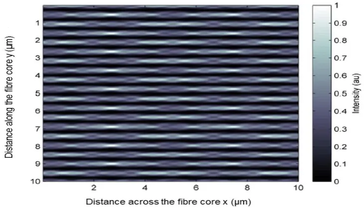
transmit more than 35% each and the rest of the transmission is via the other possible higher orders (Othonos & Kyriacos, 1999). The possibilities of fringe formation by other orders except ±1 orders have resulted in concern about how fabrication processes could impact on spectral properties. Investigation of the real structure of FBG patterns have been reported via various approaches such as: numerical analysis (Dyer, Farley & Giedl, 1995; Kouskousis et al., 2013; Mills et al., 2000; Tarnowski & Urbanczyk, 2013), experimental analysis (Rollinson et al., 2005) and microscopic analysis (Dragomir et al., 2003; Goh et al., 2014; Kouskousis, 2009; Yam et al., 2009). These analyses show how the existence of a complex FBG structure is as a result of the contribution of multiple orders and their interference. Figure 2.14 shows the modelled refractive index variation in the fibre core obtained by Kouskousis et al. (2013) considering interference of 0 - ± 4th_{orders. According to these analyses, it was observed and confirmed that}

the complex structure includes multiple periodic structures at certain distances from the phase mask which is due to the Talbot effect (discussed in the subsequent paragraph). Although the existence of complex FBG structures and how these relate to the resultant spectrum has been considered, there is need for more extensive modelling to improve our understanding.

Figure 2.14: Modelled intensity variation in the core area of the fibre due to contribution of multiple diffraction orders from phase mask fabrication (Kouskousis et al., 2013)

(50)

30

observed in atom optics. As a result of the fundamental Fresnel diffraction effect, it has gained a great attention over wide range of applications such as real time data acquisition, generation of ultra-high speed tuneable pulse source, determination of dispersion parameters of optical fibre links and a number of spectroscopic techniques (Chavel & Strand, 1984; Chen & Azana, 2005; Guigay et al., 2004; Liu, 1988a, 1988b; Mehta et al., 2006). As a result of near field diffraction and when a plane wave transmits through periodic structure, the resultant wave-front replicates the periodic structure at a certain distance. That distance is called the Talbot length (Talbot, 1836). The phenomenon of a self-imaging distance was first defined in theoretically by Rayleigh (1881) as given by:

𝑍_𝑇 = 𝜆

1 − √1 − 𝜆2 _𝛬 𝑝𝑚 2 ⁄

Equation 2.13

Later he simplified Equation 2.13 considering the relation between 𝛬_𝑝𝑚 and 𝝺

(when wavelength is considerably small); the result was Equation 2.14 as given below:

𝑍_𝑇 = 2𝛬𝑝𝑚 2

𝜆

Equation 2.14

Measurement of the Talbot length using the equation above became popular and position of Talbot planes were calculated using Fresnel-Kirchhoff diffraction and Fourier optics. However, the difficulty of measuring all Talbot planes became a disadvantage of this methodology. That was overcome by Latimer (Latimer, 1993a, 1993b, 1993c) by introducing these patterns as a multiple-slit diffraction pattern produced by conventional mechanism instead of Fourier images of the gratings.

(51)

31

further confirmed the theoretical models based on diffraction theory (Mills et al., 2000). They also explained the reason to have repeated lengths is a result of the interaction of individual diffraction orders. Mills’ further work on scanning the intensity pattern along the optical fibre produced results that were compatible with X-ray diffraction theory, which is used to describe the electric pattern field behind the phase mask. According to his explanation, the Talbot length has been simplified, as in Equation 2.15, when the numbers of diffraction orders are small:

𝑍𝑇 =

2𝜋

[(𝑘2_{− 𝑚}2_𝐺2₎1/2_{− (𝑘}2_{− 𝑛}2_𝐺2_)]

Equation 2.15

where 𝑚 and 𝑛 are integers representing the diffraction orders 𝑚 < 𝑛, and G is the unit reciprocal lattice vector which can be calculated using 2π Λ⁄ pm of the

phase mask with periodicity Λpm.

2.4.5 INDUCED REFLECTANCE AND SPECTRAL CHARACTERISTICS

The reflectivity of a grating which has constant modulation amplitude and period was explained using coupled mode theory by Lam and Garside (1981). Using coupled mode theory, which is more popular for describing the behaviour of Bragg gratings, they obtained quantitative information about the spectral dependence and diffraction efficiencies of FBGs. Therefore, the reflectivity of a uniform Bragg grating can be expressed by

𝑅(𝑙, 𝜆) = 𝛺

2_{𝑠𝑖𝑛ℎ}2_(𝑠𝑙)

∆𝑘2_{𝑠𝑖𝑛ℎ}2_{(𝑠𝑙) + 𝑠}2_{𝑐𝑜𝑠ℎ}2_(𝑠𝑙)

Equation 2.16

where 𝑅(𝑙, 𝜆) is the reflectivity of a Bragg grating which is a function of wavelength

𝜆 and grating length 𝑙. ∆𝑘 and 𝑘 are the detuning wave vector and propagation constant, which are given by 𝑘 − 𝜋 𝜆⁄ and 2𝜋𝑛₀⁄𝜆 respectively. 𝛺 is the coupling coefficient and is given by Equation 2.17:

𝛺 =𝜋𝛥𝑛 𝜆 𝑀𝑝

Equation 2.17

where 𝑀_𝑝 is the power confinement factor of the fibre core and it is expressed as:

(52)

32

where V is the normalized frequency of the fibre as given by Equation 2.4. ‘s’ can be obtained by the following equation as 𝛺 and ∆𝑘 are already known:

𝑠2 = 𝛺2− 𝛥𝑘2 Equation 2.19

At the Bragg wavelength, ∆𝑘 becomes zero. Therefore Equation 2.16 can be written as

𝑅(𝑙, 𝜆) = 𝑡𝑎𝑛ℎ2(𝛺𝑙) Equation 2.20

where 𝑙 is the length of FBG which was inscribed in an optical fibre as previously shown in Figure 2.5.

As the reflectivity is a function of grating length, an increase of the grating length increases the reflectivity. Reflectivity is also dependent on the coupling constant. Therefore, an increase of the induced index change increases the reflectivity. When broadband light propagates through the fibre having a uniform FBG, the resultant reflection peak or transmission dip is observed at the same λ, as shown by Figure 2.15 (a), and Figure 2.15 (b), respectively.

Figure 2.15: Reflection (a) and transmission (b) of uniform Bragg grating

At half of the maximum of reflectance or transmittance, the grating spectral width is defined as the Full Width at of Half Maximum (𝜆𝐹𝑊𝐻𝑀), and can be calculated

using (Othonos & Kyriacos, 1999).

𝜆_{𝐹𝑊𝐻𝑀} = 𝜆_𝐵𝑠√( 𝛥𝑛 2𝑛_𝑒𝑓𝑓)

2 + (1

𝑁)