This is a repository copy of
Testing for regularity and stochastic transitivity using the
structural parameter of nested logit
.
White Rose Research Online URL for this paper:
http://eprints.whiterose.ac.uk/103024/
Version: Accepted Version
Article:
Batley, R orcid.org/0000-0002-2487-850X and Hess, S orcid.org/0000-0002-3650-2518
(2016) Testing for regularity and stochastic transitivity using the structural parameter of
nested logit. Transportation Research Part B: Methodological, 93 (Part A). pp. 355-376.
ISSN 0191-2615
https://doi.org/10.1016/j.trb.2016.07.018
© 2016, Elsevier. Licensed under the Creative Commons
Attribution-NonCommercial-NoDerivatives 4.0 International
http://creativecommons.org/licenses/by-nc-nd/4.0/
Reuse
Items deposited in White Rose Research Online are protected by copyright, with all rights reserved unless indicated otherwise. They may be downloaded and/or printed for private study, or other acts as permitted by national copyright laws. The publisher or other rights holders may allow further reproduction and re-use of the full text version. This is indicated by the licence information on the White Rose Research Online record for the item.
Takedown
If you consider content in White Rose Research Online to be in breach of UK law, please notify us by
Testing for regularity and stochastic transitivity using the
1structural parameter of nested logit
23
Richard Batley & Stephane Hess
4
Institute for Transport Studies, University of Leeds, UK
5
6
Address for correspondence: Richard Batley, Institute for Transport Studies, 7
University of Leeds, Leeds, LS2 9JT, United Kingdom
8
Telephone: +44 (0) 113 343 1789 9
Fax: +44 (0) 113 343 5334 10
E-mail: [email protected]
11
12
Keywords: regularity, stochastic transitivity, Random Utility Model, nested logit, 13
structural parameter
14
15
Abstract 16
We introduce regularity and stochastic transitivity as necessary and well-behaved
17
conditions respectively, for the consistency of discrete choice preferences with the
18
Random Utility Model (RUM). For the specific case of a three-alternative nested logit
19
(NL) model, we synthesise these conditions in the form of a simple two-part test, and
20
reconcile this test with the conventional zero-one bounds on the structural (‘log sum’)
21
parameter within this model, i.e.
0
1
, where
denotes the structural parameter.22
We show that, whilst regularity supports the lower bound of zero, moderate and strong
23
stochastic transitivity may, for some preference orderings, give rise to a lower bound
24
greater than zero, i.e. impose a constraint
l
, wherel
0
. On the other hand, we25
show that neither regularity nor the stochastic transitivity conditions constrain the upper
26
bound at one. Therefore, if the conventional zero-one bounds are imposed in model
27
estimation, preferences which violate regularity and/or stochastic transitivity may either
28
go undetected (if the ‘true’ structural parameter is less than zero) and/or be
29
unknowingly admitted (if the ‘true’ lower bound is greater than zero), and preferences
30
which comply with regularity and stochastic transitivity may be excluded (if the ‘true’
31
upper bound is greater than one). Against this background, we show that imposition of
32
the zero-one bounds may compromise model fit, inferences of willingness-to-pay, and
33
forecasts of choice behaviour. Finally, we show that where the ‘true’ structural
34
parameter is negative (thereby violating RUM – at least when choosing the ‘best’
35
alternative), positive starting values for the structural parameter in estimation may
36
prevent the exposure of regularity and stochastic transitivity failures.
37
1. Introduction
1
As is well-established in microeconomic consumer theory, the fundamental preference
2
axioms of completeness, transitivity and continuity – taken together – permit the
3
representation of an individual’s complete preference ordering by a continuous
real-4
valued order-preserving function (Debreu, 1954). An important proposition follows from
5
Debreu; the individual is conceptualised as making consumption choices as if to
6
maximise utility. This proposition, which is the cornerstone of Neo-Classical consumer
7
theory, has been the subject of considerable interest in the behavioural economics
8
literature. A focus of this interest has been the design and implementation of
9
experiments that seek to elicit empirical support for (or refutation of) the axioms of
10
completeness, transitivity and continuity – as well as other related properties of choice
11
behaviour. Emanating from this literature, several phenomena have been identified as
12
giving rise to violations of the fundamental axioms and, by implication, violations of
13
utility maximisation.
14
The present paper is motivated by an interest in exploring analogies to the fundamental
15
preference axioms, and their empirical verification, in the alternative domain of
16
probabilistic discrete choice. The discrete choice context, where the individual chooses
17
from a finite and exhaustive set of mutually-exclusive alternatives, creates difficulties
18
for conventional Neo-Classical consumer theory. This is because the theory employs
19
marginal concepts derived using calculus; application to discrete choice has been
20
described as ‘awkward’ (McFadden, 1981 p199), and worse still ‘impossible’
(Ben-21
Akiva & Lerman, 1985 p44). In response to these difficulties, a bespoke version of
22
consumer theory has evolved, centred upon the theoretical construct of the Random
23
Utility Model (RUM)1.
24
Drawing analogy with psychophysical models of judgement and choice (Fechner,
25
1859; Thurstone, 1927; Luce, 1959), RUM was conceived by Marschak (1960) and
26
Block & Marschak (1960)2 as a probabilistic representation of the Neo-Classical theory
27
of choice. In common with the Neo-Classical theory, RUM is couched at the individual
28
level, is based fundamentally on the notion that the individual acts as if to maximise
29
utility, and (in the original ‘distribution free’ form of RUM proposed by B&M, at least) is
30
entirely supported by the notion of ordinal utility. Contrasting with Neo-Classical theory,
31
however, RUM appeals to the context of discrete choice consumption.
32
The present paper relates to three strands of extant literature, as follows.
33
1.1 Representation theorems for RUM
34
The literature on representation theorems has considered the necessity and sufficiency
35
of conditions on probabilistic choice systems (PCS) giving rise to (cardinal) utility
36
1One of the reviewers of this paper pointed out that the term ‘Random Utility Model’ (RUM) has sometimes been interpreted differently in different disciplines, and that a tighter and more contemporary terminology is ‘choice probabilities induced by strict linear orders’.See Marley & Regenwetter’s (2016) recent review of deterministic and probabilistic representations of choice, which distinguished between economic (i.e. parametric) and psychological (i.e. linear order) approaches to RUM. However, since the terminology ‘choice probabilities induced by strict linear orders’ is not common parlance in transport, this paper will remain faithful to ‘RUM’, but the reviewer’s point is worthy of mention.
functions (Debreu, 1959; Davidson & Marschak, 1959) and RUM. Focussing here on
1
representation theorems for RUM, Falmagne (1978) was first to show the necessity
2
and sufficiency of the so-called ‘B&M polynomials’3. Some years later (and apparently
3
ignorant of Falmagne’s paper until their attention was drawn to it in the course of peer
4
review), Barberá & Pattanaik (1986) re-stated Falmagne’s theorem in terms of rankings
5
rather than utility scales, which allows closer correspondence with the concept of
6
ordinal utility. More recently, Fiori (2004) contributed an elegantly concise proof of
7
Falmagne’s theorem.
8
Mindful of its origins in the cognate discipline of psychophysics, it is interesting to
9
observe that RUM has attracted interest from a multidisciplinary audience, spanning
10
several core disciplines (especially economics, psychology and mathematics), as well
11
as a raft of sectoral applications (including transport, health and the environment).
12
McFadden (2005) presented a useful synthesis of representation theorems for RUM
13
and, reflecting his parent discipline of economics, he characterised such theorems as
14
addressing the ‘problem of revealed stochastic preference’4. Within this synthesis,
15
McFadden & Richter’s (unpublished) 1970a and 1970b papers, subsequently
16
consolidated within their 1991 paper, covered similar ground to Falmagne (1978).
17
Reflecting back some years later, Marley (1990) described the evolution of the
18
literature on representation theorems for RUM, and offered specific observations
19
concerning the links between the Falmagne and McFadden/Richter bodies of work.
20
A distinct but related strand of literature is that dealing with representation theorems
21
for ‘parametric’ versions of RUM5. Motivated by an interest in its practical applicability,
22
three independent parallel teams – namely Daly & Zachary (1976, subsequently
23
published in 1978), Williams (1977) and McFadden (1978) – proposed alternative
24
presentations of RUM, each formalised in terms of necessary and sufficient conditions
25
on choice probabilities and/or random utilities giving rise to choice probabilities. In this
26
context, and drawing similarities with McFadden’s ‘problem of revealed stochastic
27
preference’, the probabilistic content of RUM derives from the propensity for variability
28
in behaviour across a population of individuals, as distinct from the intra-individual
29
variability of a single individual in B&M. This change in emphasis, together with the
30
extended theoretical apparatus, provided the stimulus for the adoption of RUM in
31
mainstream econometric practice (see section 1.3 to follow).
32
1.2 Empirical testing of theoretical properties of choice
33
Following from the theoretical developments outlined above, a second strand of
34
literature has subjected the fundamental preference axioms – as well as a broader
35
range of theoretical properties of choice – to empirical testing. In this context, the
36
psychology and behavioural economics literatures would seem rather more developed
37
than the discrete choice literature, but this perhaps reflects the relative infancy of the
38
3 See Theorem 4 (p60) of Falmagne (1978).
4 According to McFadden (2005), this problem poses the question: ‘Are the distributions of choices observed for a population of individuals in a variety of choice situations consistent with rational choice theory, which postulates that individuals maximize preferences?’ (p245).
5 In this regard, Regenwetter et al (2010) distinguished between B&M’s ‘distribution free’ RUM and the
latter. Following the conception of non-parametric RUM in 1960, parametric versions
1
of RUM entered practical usage only in the late 1960s; see McFadden’s 1968 (but
2
unpublished until 1975) pioneering application to public policy analysis. Despite their
3
different levels of maturity, the psychology, behavioural economics and discrete choice
4
literatures show interesting parallels in terms of the phenomena which have been
5
observed in experimental contexts (for a recent overview of this literature, see
6
Busemeyer & Rieskamp, 2013). Of particular relevance to the present paper are three
7
phenomena, namely ‘regularity’, ‘transitivity’ and ‘invariance’. These phenomena will
8
be formally analysed in sections 2 and 3 to follow; the present section simply introduces
9
the intuition for each phenomenon, and briefly summarises their respective evidential
10
positions.
11
Regularity: this property asserts that the probability of choosing any given alternative 12
from an offered set should not increase if the offered set is expanded to include
13
additional alternatives. Violations of regularity were first reported by Huber et al (1982),
14
who rationalised these violations in terms of ‘asymmetric dominance’. The latter
15
phenomenon characterises situations where a binary choice set is appended by a third
16
alternative which is similar – but materially inferior – to one of the initial pair. According
17
to asymmetric dominance, the third alternative is rarely chosen, but its inclusion in the
18
offered set enhances the probability of choosing the similar alternative from the initial
19
pair. Whilst different explanations for asymmetric dominance have been advanced in
20
the literature (e.g. Simonson, 1989; Simonson & Tversky, 1992), there is reasonable
21
consensus that this phenomenon is prevalent in choice experiments (Heath &
22
Chatterjee, 1995). More generally, there exists an extensive mature literature in
23
psychology on choice and response time for so-called ‘context effects’, where choice
24
is affected by the presence or absence of other alternatives. Within this literature, the
25
similarity between alternatives has been identified as a principal context effect (e.g.
26
Trueblood et al, 2015).
27
Transitivity: this property asserts that if alternative
x
is preferred to alternativey
,28
and
y
toz
, thenx
should be preferred toz
. Recognising that transitivity is29
ostensibly a deterministic property, the RUM literature has developed various
30
stochastic interpretations of transitivity (referred to as ‘weak’, ‘moderate’ and ‘strong’).
31
None of these variants of transitivity are necessary for RUM, although there is a close
32
relationship between stochastic transitivity and the so-called ‘triangle condition’ (see
33
section 2.2 to follow), which is necessary for RUM. Following the precedent of
34
Papandreou (1957) and Davidson & Marschak (1958)6, researchers have subjected
35
stochastic transitivity to empirical testing, and have generally reported evidence of
36
violations (see Rieskamp et al (2006) and Hougaard et al (2011) for overviews of this
37
literature). However, the recent paper by Regenwetter et al (2011) systematically
38
reanalysed much of this evidence; using a non-parametric statistical test of the triangle
39
condition, they found that most individuals did not produce statistically significant
40
violations. More recently, Cavagnaro & Davis-Stober (2014) repeated the same
41
analysis using a slightly refined version of Regenwetter et al’s test; this revealed
42
variability in stochastic transitivity properties across individuals, but essentially
43
corroborated Regenwetter et al’s finding.
44
Invariance: this property asserts that the relative preference between two alternatives 1
should be invariant to the addition/subtraction of other alternatives to/from the choice
2
set. An important feature of early discrete choice model specifications was the
3
‘Independence from Irrelevant Alternatives’ (IIA) property (Luce, 1959), which states
4
that the ratio of any two choice probabilities is unaffected by the presence or absence
5
of other alternatives in the choice set. Modellers initially saw IIA as an attractive
6
property, in the sense that the choice between alternatives could be predicted without
7
the need for data on ‘external’ alternatives, and this prompted widespread application
8
of the multinomial logit (MNL) model (McFadden, 1973). Subsequently, IIA began to
9
be seen more as a weakness rather than a strength, since it was unable to account for
10
similarity between alternatives, which had been identified as an important determinant
11
of choice (Tversky, 1972a; 1972b).
12
This prompted the development and adoption of the nested logit (NL) model (Daly &
13
Zachary, 1976; Williams, 1977)7, which generalises MNL such that subsets of similar
14
alternatives are ‘nested’ together, not unlikeTversky & Sattath’s (1979) concept of a
15
preference tree (or PRETREE)8. McFadden (1978) formalised the specification of
16
parametric RUM models through the Generalised Extreme Value (GEV) theorem. GEV
17
gives rise to a subset of models within the RUM class (Ibáñez, 2007), which embody
18
general patterns of correlation between alternatives, and include MNL and NL among
19
its members. Throughout the 1980s and 1990s, MNL and NL established themselves
20
as the primary tools of discrete choice modellers; for example Ortúzar (2001) described
21
them as the ‘…the workhorses for the empirical analysis of travel behaviour in respect
22
of discrete choices’ (p213). This did not however deter the exploration for further
23
generalisations of RUM, especially in terms of the flexibility of substitution patterns
24
between discrete choice alternatives. Cross-nested logit (CNL), which is also derived
25
from GEV, generalises NL by allowing alternatives to belong to more than one nest,
26
potentially with different ‘degrees’ of membership. Although the derivation of CNL is
27
usually credited to Vovsha (1997), the model was clearly stated in Williams (1977) and
28
McFadden (1978). Swait’s (2001) GenL model, which is motivated by a specific interest
29
in choice set generation, restricts CNL by suppressing the different degrees of
30
membership. Daly and Bierlaire’s Recursive Nested Extreme Value (RNEV) model
31
(Daly, 2001; Bierlaire, 2002; Daly & Bierlaire, 2006) generalises both NL and CNL, by
32
allowing cross-nesting with an arbitrary number of levels.
33
1.3 The feasible range of the structural parameter in GEV
34
Having exposed the key role played by the invariance property within practical
35
specifications of RUM, let us now consider the ability to test observed behaviour for
36
consistency with RUM. In this regard, the structural parameter
of the GEV-based37
models (MNL, NL, CNL and RNEV), otherwise referred to as the coefficient of the
38
‘inclusive value’ within these models, will be the focus of our interest. Conventional
39
practice is to constrain the choice model in estimation such that the structural
40
parameter falls within the bounds
0
1
. Informing this convention, McFadden41
7 Building upon earlier contributions by Manheim (1973), Wilson (1974) and Ben-Akiva (1974); see the
historical account in Ortúzar (2001).
(1981) remarked (but did not prove) that: ‘A necessary and sufficient condition for [NL]
1
to be consistent with GEV is that…the coefficient of each inclusive value…lie[s] in the
2
unit interval’ (p240). In support of the zero-one bounds, McFadden presented two
3
arguments, one rationalising the structural parameter in terms of correlation between
4
nested alternatives, and a second based upon testable properties of binary choice
5
data; the latter argument is considered more fully in Annex B of the present paper.
6
With regards to the lower bound of the structural parameter in GEV models, Train
7
(2003) remarked that: ‘A negative value of [the structural parameter] is inconsistent
8
with utility maximisation and implies that improving the attributes of an alternative (such
9
as lowering its price) can decrease the probability of it being chosen’ (p81). McFadden
10
(1981) further remarked: ‘It should be noted that, while a negative coefficient of
11
inclusive value leads to a local failure of the GEV conditions, a coefficient of an
12
inclusive value exceeding one will fail to satisfy GEV only for some values of the
13
variables. Thus it is possible that an empirical fit yielding a coefficient greater than one
14
will be consistent with GEV over the range of the data and can be combined with a
15
second function outside the range of the data to yield a system that satisfies GEV
16
globally. However, this chapter has not attempted to develop a test for local
17
consistency with GEV at the observations, or for consistency with some function that
18
satisfies GEV globally’ (p248).
19
With regards to the upper bound of the structural parameter in GEV models, a number
20
of researchers have reviewed the practical convention of constraining
1
, further21
developing McFadden’s (1981) points noted above. The initial contribution in this
22
regard was by Börsch-Supan (1990), who sought to demonstrate that, for two-level NL,
23
1
is consistent with RUM for some range of (but not all) values of the explanatory24
variables. In this way, Börsch-Supan admitted the possibility of more flexible ‘local’
25
bounds on the structural parameter, whilst complying with the conventional zero-one
26
bounds in a ‘global’ sense. As evidential support, Börsch-Supan cited examples from
27
the literature of NL models exhibiting
1
, namely Börsch-Supan (1985), Hensher28
(1984) and Small & Brownstone (1982). Train (2003) cited the additional examples of
29
Train et al (1987) and Lee (1999). In these cases,
1
was accepted by the30
respective authors as a valid result, and interpreted as reflecting greater substitutability
31
between nests than within nests. Herriges & Kling (1996), building upon Koning &
32
Ridder (1994), subsequently corrected an oversight in Börsch-Supan, and offered
33
proof of the definitive conditions on the structural parameter for two-level NL involving
34
nests of two, three or four alternatives. They further applied the model empirically,
35
showing the dependence of these conditions on the marginal probabilities of choosing
36
the nests. For the simplest case of two-level NL involving nests of two alternatives –
37
which will be the focus of the present paper – Herriges & Kling calculated an upper
38
bound on the structural parameter of 20 for consistency with RUM. This result was
39
however associated with an extreme marginal probability of 0.95; for a marginal
40
probability of 0.5, the upper bound was reduced to 2, and for lower marginal
41
probabilities still, the permissible range showed little increase beyond 1.
42
In the course of a comprehensive review of NL, Carrasco & Ortúzar (2002, section 3.5)
43
devoted particular attention to the bounds of the structural parameter, identifying some
44
practical limitations of the Börsch-Supan’s (1990) argument (and its subsequent
45
well be sub-optimal in terms of explanatory fit. Second, the admission of
1
may1
contravene the requirement for a decreasing structural parameter (and by implication
2
an increasing scale) as one moves down multi-level NL. Third, whilst the Börsch-Supan
3
argument has theoretical credence, it has received limited support from empirical
4
evidence. Moreover, as a preamble to their review, Carrasco & Ortúzar (2002, section
5
2.3) compared and contrasted the alternative derivations of NL developed by Williams
6
(1977) and McFadden (1978), and in particular highlighted their different rationales for
7
the structural parameter. Williams’ (1977) alternative derivation of NL represents the
8
structural parameter as the ratio of scale parameters at adjacent levels of the tree,
9
where the scale parameters reflect the variance of the random terms at the respective
10
levels. The implication of this derivation is that –unlike McFadden’s NL –Williams’ NL
11
constrains the structural parameter to the zero-one bounds, and requires the structural
12
parameter to increase as one moves down the tree. Furthermore, with reference to the
13
earlier justification for GEV-based NL models exhibiting
1
, Williams’ NL in effect14
constrains patterns of substitution between alternatives (Williams & Senior, 1978).
15
1.4 The contributions of the present paper
16
The present paper does not seek to revisit the question of how the
0
1
bounds17
relate to the definition of RUM per se (whether in the context of McFadden’s or
18
Williams’ derivations), but instead addresses the more general question of how these
19
bounds relate to the properties of regularity and stochastic transitivity introduced in
20
section 1.2 above. However, as will be apparent from the summary of literature above,
21
any interest in the
0
1
bounds is intertwined with interests surrounding22
representation theorems for RUM and the invariance property. Whilst B&M showed
23
that stochastic transitivity – unlike regularity – is unnecessary to derive RUM, our
24
interest in this property is motivated by the proposition that any ‘well-behaved’ discrete
25
choice model might be expected to exhibit stochastic transitivity.
26
Against this background, the present paper offers three principal contributions:
27
1. We will distinguish between necessary (which we represent in terms of
28
regularity) and well-behaved (which we represent in terms of stochastic
29
transitivity) conditions for RUM.
30
2. Focussing specifically upon three-alternative NL, we will synthesise these
31
necessary and well-behaved conditions for RUM in the form of a simple
two-32
part test.
33
3. Using both theory and empirics, we will reconcile the simple two-part test with
34
conventional criteria for determining the RUM-compliance of three-alternative
35
NL.
36
To these ends, the layout of the paper is as follows. Section 2 presents a formal
37
definition of RUM, details the theoretical conditions which give rise to this definition,
38
and arising from these conditions identifies properties which will be the subject of
39
empirical testing. Section 3 describes, in analytical terms, the application of these tests
40
to a special case of RUM in the form of two-level NL. In order to illustrate the practical
41
implication of section 3, section 4 develops broadly the same example empirically,
42
using both simulated and real data. Section 5 provides a summary and conclusion.
43
2. Theoretical background of RUM
1
2.1 Theoretical conditions underpinning RUM
2
Consider an individual economic agent, who is offered a finite and exhaustive set of
3
mutually exclusive alternatives:
4
1,...,
N
n
5
Let us further restrict the analysis to a feasible subset
M
N
, which we refer to as6
the ‘choice set’. We will not concern ourselves with the specific constraints determining
7
feasibility, but these could include factors such as budget. B&M9 introduced two
8
‘conditions’ (their terminology) which define RUM, thus10:
9
CONDITION
P
, Rankings consistent with the Random Utility Model: There are n! 10numbers
p r
such that for any xM and any M,M
N
:11
0
p r
and
; x M
M R
p
x
p r
12where
p r
is the probability of the rankingr
; Rx M; is the set of all rankingsr
on M 13for which
x
is the first among all elements of M, i.e.R
x M;
r r
x
r
y
for all yM 14; and
p
M
x
is the probability of alternativex
being chosen from M, where15
0
p
Mx
1
and M
1
x M
p
x
.16
Whilst the above condition encompasses all preference orderings on the feasible set,
17
the condition that follows considers the subset of preference orderings where a given
18
alternative is first ranked (i.e. is chosen).
19
CONDITION
U
, Random Utility Model: There is a random vector
U
1,...,
U
n
unique20
up to an increasing monotone transformation such that for any xM and any M,
21
M
N
:22
Pr
M x y
p x U U for all yM 23
If the random utilities are (uniformly) continuous random variables, then this implies
24
non-coincidence, i.e. Pr
Ux Uy
0 for all yM. On this basis, Condition
U
25effectively defines the existence of a probability space on these random utilities.
26
9This section adheres closely to B&M’s seminal 1960 paper, and the reader is referred to that paper for more detailed discussion of the various definitions and conditions. However, much of the same material is covered by Fishburn’s (1998) subsequent and very authoritative review.
10 In what follows, we deploy the following notational conventions to represent choice probability, namely:
M
p x is the probability of choosing x from the offered set M;
, , x y z
Finally, note that B&M (Theorem 3.1, p183) showed that conditions
U
and
P
each1
imply the other, i.e.
U
P
11.2
2.2 Theoretical conditions as testable properties of RUM
3
In seeking to confirm the consistency (or otherwise) of given data with RUM, it should
4
be acknowledged that: ‘...save for the choice axiom, [models of the RUM class] are all
5
stated in terms of nonobservable utility functions, and so it is impossible to test them
6
completely until we know conditions that are necessary and sufficient to characterize
7
them in terms of preference probabilities themselves, for only these can be estimated
8
from data’ (Luce & Suppes, 1965 pp339-340). Contemporary discrete choice modellers
9
have tended to overlook B&M’s original work on RUM, which devoted detailed attention
10
to testable properties and defined several conditions which follow from
U
and
P
11. These conditions refer to various properties of binary and multinomial choice
12
probabilities on the feasible set M , as follows.
13
CONDITION
e
, Regularity: If LM, thenp
M
x
p
L
x
for allx
L M
,
, LM 14CONDITION
e
3 , Regularity for any trinary: For any three elements x y z, , M,15
x y z, ,
,
p
x
p x y
, or equivalently px y z, ,
x min
p x y
,
,p x z,
16B&M (Theorem 3.3, p185) showed that condition
P implies condition
e
, which itself17
implies (but is not implied by) condition
e
3 , i.e.
P
e
e
3 . In general,18
regularity is necessary but not sufficient for RUM (Marschak, 1960, p192), but in the
19
specific case of a trinary choice set, regularity is necessary and sufficient for RUM to
20
hold. Some additional conditions follow:
21
CONDITION
c
3 , Triangular condition: For any three distinct elements x y z, , M 22
1
p x y
,
p y z
,
p z x
,
2
23It is well known that for binary choice probabilities involving up to five distinct
24
alternatives, RUM holds if and only if the relevant triangle inequalities hold (Cohen &
25
Falmagne, 1971; 1990; McFadden & Richter, 1970a; 1970b; 1991; Fishburn, 1998;
26
Cavagnaro & Davis-Stober, 2014). B&M (Theorem 5.6, p195) and Luce & Suppes
27
(1965, Theorem 34, p343) further showed that
e
3c
3 .28
2.3 Other theoretical conditions as testable properties
29
The above relations reveal that regularity is the key condition for testing the
30
consistency of discrete choice preference data with RUM. However, Marschak (1960)
31
described the following conditions as ‘...partial results (which) may, however, prove
32
useful’.
33
11 In what follows, we use to denote ‘implies’, to denote ‘implies and is implied by’, and to
CONDITION
WST
, Weak Stochastic Transitivity: If
,
1
2
p x y
and1
,
1
2
p y z
, then
,
1
2
p x z
2CONDITION
MST
, Moderate Stochastic Transitivity: If
,
1
2
p x y
and3
,
1
2
p y z
, then p x z
, min
p x y p y z
, , ,
4CONDITION
SST
, Strong Stochastic Transitivity: If
,
1
2
p x y
and5
,
1
2
p y z
, then p x z
, max
p x y p y z
,
, ,
6Marschak (1960; Theorem 12, p227) showed that
SST
MST
WST
,7
whilst B&M (Theorem 5.8, p196) showed that
SST
c
3 , and Luce & Suppes8
(1965; Theorems 35 and 38, pp343-346) showed that
MST
c
3 .9
10
3. An analytical example
11
Following from the preceding discussion, any test of regularity on a given trinary (i.e.
12
condition
e
3 ) amounts to a comparison of the binary and trinary choice probabilities13
and, in particular, an examination of how these probabilities deviate depending upon
14
the presence/absence of a ‘third’ alternative. Regularity will certainly hold in discrete
15
choice contexts subject to IIA, but may not hold otherwise. Since the NL model
16
(Williams, 1977; Daly & Zachary, 1978; McFadden, 1978) seeks to relax IIA, an
17
interesting question is whether NL complies with regularity; this question will be the
18
focus of section 3.3.1.
19
Although stochastic transitivity – unlike regularity – is not a necessary condition of
20
RUM, we hypothesise that any ‘well-behaved’ discrete choice model will exhibit MST
21
or (better still) SST. We further hypothesise that, by ensuring compliance with MST
22
and SST, modellers will yield RUMs that embody more intuitive parameter estimates
23
(e.g. in terms of the size and sign of implied demand elasticities), and greater
24
explanatory power. In a similar fashion to our analysis of regularity, section 3.3.2 will
25
consider the extent to which NL complies with stochastic transitivity.
26
Before embarking upon these discussions of regularity and stochastic transitivity,
27
section 3.1 will introduce an illustrative choice problem, and section 3.2 will apply NL
28
to this problem. In considering the compliance of NL with regularity and stochastic
29
transitivity, a key focus will be whether these conditions corroborate the conventional
30
0
1
bounds on the structural parameter.31
3.1 The choice problem
32
In testing the compliance of RUM with the fundamental preference axioms, behavioural
33
economists have tended to adhere to B&M’s original definition of RUM, which
interprets U as a random ordinal variable. By contrast, discrete choice modellers have
1
re-interpreted U as a random cardinal variable, via the following definition:
2
x x x
U
V
for allx
M
(1)3
where
V
x are constants referred to as ‘deterministic utility’, and
x are random4
variables exogenous12 of x
V
with a continuous joint finite density function. This defines5
the class of Additive Random Utility Models (ARUM).
6
Henceforth, we restrict the scope of the paper to the case where the choice set consists
7
of the trinary13:
8
, ,
M
x a b
N
9wherein
a
andb
show some degree of similarity not possessed byx
. For example,10
in the case of travel mode choice,
a
andb
could represent two alternative bus11
services to a given location, whilst
x
could represent car. Reflecting these features,12
let us create a subset containing the two similar (i.e. bus) alternatives
a
andb
:13
,
L
a b
M
14The NL model arises from a special case of (1) where the random variables for all three
15
alternatives are identically Gumbel distributed, but where
a and
b (e.g. the random16
variables for the bus alternatives) are correlated with each other, whilst
x (e.g. the17
random variable for the car alternative) is independent of
a and
b. The correlation18
between
a and
b seeks to capture the degree of similarity betweena
andb
.19
3.2 A nested logit representation of the choice problem
20
Following McFadden (1987), a NL representation of the aforementioned choice
21
problem is uniquely determined by two choice probabilities, namely the marginal
22
probability of choosing
L
M
:23
ln
ln
Va Vb
Va Vb
x e e
M
e e
V
e p L
e e
(2)
24
and the conditional probability of choosing
a
L
:25
12 This assumption of exogeneity is almost unavoidable if there is wish to apply RUM to welfare analysis; see McFadden (1995) or Batley (2014).
13 The three-alternative choice set is but one example of real world or experimental choices. However, it
,a
a b V
L V V
e p a p a b
e e
(3)
1
where
continues to denote the structural parameter, and the model is implicitly upper2
normalised (Hensher & Greene, 2002; Carrasco & Ortúzar, 2002). Drawing reference
3
to Carrasco & Ortúzar’s critique of Börsch-Supan (1990), which was summarised in
4
section 1.3 above, note that (2) and (3) give rise to two-level NL, thereby avoiding any
5
complications associated with multiple levels.
6
In these terms, the probabilities of choosing the similar alternatives
a
andb
are given7
by:
8
,
M M
p
a
p
L
p a b
9
1
,
M M
p
b
p
L
p a b
10whilst the probability of choosing the dissimilar alternative
x
is given by:11
1
M M
p
x
p
L
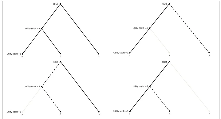
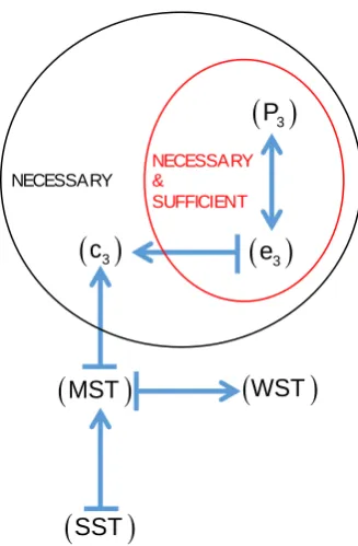
12This tree structure is illustrated in the top left panel of Figure 1.
13
FIGURE 1 ABOUT HERE
14
3.3 Applying the testable properties to three-alternative nested logit
15
Again drawing from B&M’s derivation of the theoretical conditions, but now focussing
16
on the trinary choice set (and employing the notation
P
3 to represent the application17
of condition
P
to this trinary set and all of its non-empty subsets), the testable18
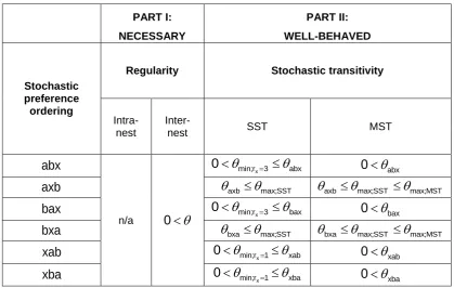
properties from section 2 above are summarised in Figure 2.
19
FIGURE 2 ABOUT HERE
20
An important practical property of NL (and indeed of any parametric RUM) is that,
21
having established a model on the complete choice set M, it readily lends itself to the
22
derivation of choice probabilities for any reduced choice (i.e. for any subset of M).
23
This property, which avoids the need to systematically model the full permutation of
24
preference orderings, will be exploited in what follows. We will return to this point when
25
introducing the empirical example in section 4.
26
3.3.1 Compliance with regularity
27
In testing compliance with the regularity condition, two general cases are of relevance.
28
Case 1: Intra-nest choice 29
For the three alternative NL choice problem under examination, regularity is satisfied
30
if both:
31
,
M
With reference to Annex A, it is trivial to show that, for intra-nest choice, compliance
1
with regularity is guaranteed, irrespective of the value taken by the structural parameter
2
.3
Case 2: Inter-nest choice 4
In this case, regularity is satisfied if:
5
,
M
p x a
p
x
,p a x
,
p
M
a
,p x b
,
p
M
x
, andp b x
,
p
M
b
6For inter-nest choice, Annex A further shows that compliance with regularity will
7
depend upon the relative magnitudes of the marginal and conditional probabilities14. In
8
particular, negative values of the structural parameter are non-compliant, but values
9
greater than one could be compliant.
10
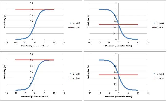
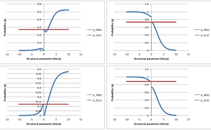
Drawing together Cases 1 and 2 above, Figures 3 and 4 provide an empirical example
11
of the choice problem under examination. Whilst Figure 3 assumes
V
a
V
b
V
x, such12
that the three alternatives are deterministically indifferent, Figure 4 assumes
13
9,
8,
10
a b x
V
V
V
, such thatx
is deterministically preferred toa
,a
tob
, and14
x
tob
. In both figures, the upper and lower panels compare, for each of the inter-nest15
choices, the binary and multinomial choice probabilities as the structural parameter is
16
increased from -10 to +10. With reference to (1), the structural parameter effectively
17
represents the magnitude and interdependence of the random variables for the three
18
alternatives. Despite the differences in deterministic preferences, both figures
19
corroborate our theoretical proposition that regularity requires
0
, since at negative20
values of the structural parameter one or more of the binary choice probabilities are
21
less than their associated multinomial choice probabilities. Furthermore, in the case of
22
Figure 4, regularity also gives rise to an upper bound, since
p b x
,
p
M
b
where23
1.5
.24
FIGURE 3 ABOUT HERE
25
FIGURE 4 ABOUT HERE
26
3.3.2 Compliance with stochastic transitivity
27
Relative to the discussion of regularity above, the discussion of stochastic transitivity
28
will require rather more exposition. With reference to the general case outlined in
29
section 2.3 above (i.e. not specific to NL), we begin by introducing the notation
xyz
to30
represent a complete set of binary stochastic preferences on the trinary choice set
31
x y z
, ,
such thatp x y
,
1 2
,p y z
,
1 2
andp x z
,
1 2
. In other words,32
xyz
represents a preference ordering that complies with WST as a minimum (and33
possibly also complies with MST and SST)15.
34
14This dependence resonates with Herriges & Kling’s (1996) findings reported in section 1.
15 As pointed out by one of the anonymous reviewers of this paper, xyz does not in general imply
M M M
Now relating this notation to the specific case of the three alternative NL under
1
examination here, we refer to axb as the intrinsic preference ordering, on the grounds
2
that the first two stochastic binary choices in the transitivity chain (i.e. the inter-nest
3
binary choices between
a
andx
(see top right panel of Figure 1), and betweenx
4and
b
(see bottom left panel of Figure 1)) will be independent of the value of the5
structural parameter, whilst the final stochastic ‘transitive’ choice (i.e. the intra-nest
6
binary choice between
a
andb
(see bottom right panel of Figure 1)) will be dependent7
on the value of the structural parameter16.
8
Following the rationale outlined in Annex B, the intrinsic preference ordering allows us
9
to infer, for given inter-nest binary choices, the upper bound on the structural
10
parameter such that the intra-nest binary choice complies with stochastic transitivity,
11
thus:
12
ln 1
1
ln 1
u
v
w
(4)13
where:
14
,
,
1
p a x
p x a
u
15
,
,
1
p x b
p b x
v
16,
0
u v
17and:
18
,
,
1
p a b
p b a
w
19
max
,
w
u v
in the case of SST20
min
,
w
u v
in the case of MST21
0
w
in the case of WST22
That is to say, conditional upon
a
being stochastically preferred tox
, andx
tob
, (4)23
elicits the upper bound on
which ensures thata
is stochastically preferred tob
with24
sufficient strength that stochastic transitivity holds for the intrinsic preference ordering
25
axb
. Since MST is associated with the minimum value ofw
, and SST is associated26
with the maximum, these two transitivity conditions may give rise to different upper
27
bounds on the structural parameter.
28
Having derived (4) for the intrinsic preference ordering
axb
, let us now consider its29
application as a test of stochastic transitivity for actual preference orderings covering
30
all possibilities. To this end, two general cases are of relevance, depending on whether
31
16 This definition of the intrinsic preference ordering resonates with Herriges & Kling’s (1996) comment:
the ‘transitive’ choice (i.e. the final binary choice of the actual preference ordering) is
1
intra-nest (i.e. in the manner of the intrinsic preference ordering) or inter-nest17.
2
Case 3: Where the ‘transitive’ choice is intra-nest 3
This case deals with actual preference orderings axb and bxa (again reflecting
4
complete binary stochastic preferences on the trinary choice set, as per the notational
5
definition at the beginning of section 3.3.2). However, having defined the discrete
6
choice problem (section 3.1), and determined which alternatives should be nested
7
together (section 3.2), it is arbitrary as to whether a given nested alternative is labelled
8
a
orb
. The implication follows that the same bounds on the structural parameter will9
(in essence18) apply to the actual preference orderings axb and bxa. Moreover, Case
10
3 is in substantive terms consistent with the intrinsic preference ordering, and
11
focussing here upon axb, we can re-state (4)19:
12
maxln 1 1 ln 1 1
ln 1 ln 1
axb
axb
u v u v
w w k
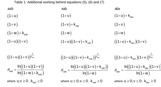
(5)
13
where
k
axb is a non-negative constant (see Table 1 for additional working). From (5)14
we can infer that:
15
SST entails an upper bound on the structural parameter, which we denote
16
max;SST
, and which may be greater than one.17
MST also entails an upper bound, which we denote
max;MST, and which may18
itself be greater than
max;SST.19
In summary:
axb
max;SST
max;MST.20
A corollary of the above findings is that (5) will elicit the conventional upper bound of
21
one for the structural parameter only where
a
and/orb
is indifferent tox
20.22
To give these results some intuition, note that whilst the inter-nest binary probabilities
23
(which in Case 3 account for the first and second choices in the transitivity chain) will
24
be independent of the value of the structural parameter, the intra-nest binary probability
25
(which in Case 3 accounts for the third ‘transitive’ choice) will not. For this case, we
26
17 In passing, it is worth remarking that we confirmed the bounds for both Cases 3 and 4, by applying the stochastic transitivity tests (B1), (B2) and (B3) to a wide range of values for both the deterministic utilities (i.e. V V V ) and the structural parameter (i.e. x, a, b ), and checking correspondence with the bounds on
the structural parameter arising from (5), (6) and (7).
18 With the caveat that, having adopted a given intrinsic preference ordering (either axb or bxa ),
max( , )
w u v and wmin( , )u v for the actual preference ordering axb will correspond to min( , )
w u v and wmax( , )u v respectively for the actual preference ordering bxa .
19 A slight qualification is that we introduce the subscript axb to the structural parameter to denote the actual preference ordering; we will adopt the same convention in the subsequent working.
20 In this case, from (B10) it must hold that
1w
1 u
1v
, which simplifies to w u v uv.wish to discern, for given inter-nest binary probabilities greater than 0.5, any bounds
1
on the structural parameter which ensure that the intra-nest binary choice will complete
2
the transitivity chain. Since an increasing value of the structural parameter will amplify
3
the probability of choosing the (deterministically) inferior alternative from the intra-nest
4
binary, Case 3 gives rise to an upper bound on the structural parameter; at higher
5
values of the structural parameter, the (deterministically) inferior intra-nest alternative
6
will become sufficiently attractive that stochastic transitivity fails. Consider for example
7
the actual preference ordering axb. If the inter-nest choices are consistent with this
8
preference ordering (i.e.
a
is stochastically preferred tox
, andx
tob
), then9
compliance with stochastic transitivity rests upon the intra-nest choice, in particular the
10
strength of preference for
a
overb
, relative to the strength of the inter-nest11
preferences. An increasing value of the structural parameter will gradually reduce the
12
intra-nest probability for
a
overb
, until an upper bound is reached where stochastic13
transitivity fails.
14
Case 4: Where the ‘transitive’ choice is inter-nest 15
Whereas Case 3 dealt with actual preference orderings that are consistent with the
16
intrinsic preference ordering, in the sense that the ‘transitive’ choice is intra-nest, Case
17
4 deals with actual preference orderings that entail inter-nest transitivity, i.e. abx,
18
bax, xab and xba (again reflecting complete binary stochastic preferences on the
19
trinary choice set, as per the notational definition at the beginning of section 3.3.2). As
20
was noted in Case 3 however, having determined which alternatives should be nested
21
together, it is arbitrary as to which alternative is labelled
a
andb
. In practice,22
therefore, we need only consider two of these four preferences orderings, where the
23
defining feature of these preference orderings is the rank of the lone alternative
x
.24
Case 4.1: Consider the actual preference ordering xab, where the lone alternative is
25
first-ranked (i.e.
r
x
1
, noting that we could instead consider xba, and (in essence21)26
derive the same bounds on the structural parameter). Reconciling xab with the odds
27
ratios (B4a) and (B4b), we can reason that (see Table 1 for additional working), in the
28
case of the actual preference ordering xab, it must hold that
p a x
,
p x a
,
1
,29
,
,
1
p x b
p b x
andp a b
,
p b a
,
1
. The implication is that, whereas Case30
3 gave rise to an upper bound on the structural parameter (5), the present case gives
31
rise to the lower bound:
32
min; 1ln 1
1
ln 1
1
ln 1
ln 1
xxab
xab r
u
v
k
u
v
w
w
(6)33
21 In an analogous fashion to Case 3, having adopted an intrinsic preference ordering (either axb or bxa
), wmax( , )u v and wmin( , )u v for the actual preference ordering xab will correspond to
min( , )
where min; 1
x r
denotes the lower bound of the structural parameter given that the lone1
alternative is ranked first,
u
0
,v
0
,w
max
u v
,
for SST,w
min
u v
,
for2
MST, and
k
xab
0
.3
TABLE 1 ABOUT HERE
4
It should be qualified that, given the relations inherent within (6), the lower bound for
5
MST will in principle be negative (more specifically, the numerator of the lower bound
6
in (6) will be positive, but the denominator will be negative). In practice however, a
7
negative structural parameter will violate regularity (section 3.3.1), and it therefore
8
makes sense to impose a lower bound of zero for MST.
9
Case 4.2: Consider the actual preference ordering abx, where the lone alternative is
10
third-ranked (i.e.
r
x
3
, noting that bax will (in essence22) yield the same bounds on11
the structural parameter). Following an analogous line of reasoning to Case 4.1, it must
12
in this case hold that
p a x
,
p x a
,
1
,p x b
,
p b x
,
1
and13
,
,
1
p a b
p b a
, thereby giving rise to the lower bound:14
min; 3ln
1
1
ln 1
1
ln 1
ln 1
xabx
abx r
u
k
v
u
v
w
w
(7)15
where min; 3
x r
denotes the lower bound of the structural parameter given that the lone16
alternative is ranked third,
u
0
,v
0
,w
max
u v
,
for SST,w
min
u v
,
for17
MST, and
k
abx
0
. In practice, the lower bound for MST will again be zero.18
Moreover (6) and (7) provoke the following inferences:
19
In summary:
0
min; 3x
r abx
, and0
min; 1x
r xab
20
Whether min; 1 min; 3
x x
r r
, or
min;rx1
min;rx3, will be an empirical issue.21
To give this result some intuition, in Case 4 the intra-nest choice will be first or second
22
in the transitivity chain, whilst the third (i.e. ‘transitive’ choice) will be inter-nest. As
23
before, we wish to discern, for given inter-nest probabilities, any bounds on the
24
structural parameter such that the intra-nest probability (which unlike Case 3 will not
25
be the third ‘transitive’ choice) is consistent with the transitivity chain. Consider for
26
example the actual preference ordering abx. If the inter-nest choices are consistent
27
with this preference (i.e. a is stochastically preferred to
x
, and b tox
), then28
compliance with stochastic transitivity rests upon the intra-nest choice, in particular the
29
strength of preference for a over b, relative to the strength of the inter-nest
30
preferences. As the value of the structural parameter increases, the probability of
31
choosing a over b will decrease, whilst the probability of choosing a over
x
will32
22 In an analogous fashion to Case 3, having adopted an intrinsic preference ordering (either axb or bxa
), wmax( , )u v and wmin( , )u v for the actual preference ordering abx will correspond to
min( , )