R E S E A R C H
Open Access
Dynamics analysis for a discrete dynamic
competition model
Xiuqin Yang
1, Feng Liu
2*, Qingyi Wang
2and Hua O. Wang
3*Correspondence:[email protected] 2School of Automation, China
University of Geosciences, Wuhan, P.R. China
Full list of author information is available at the end of the article
Abstract
In this paper, the dynamics of a discrete market share attraction model are investigated. It shows that the system can undergo flip bifurcation and chaos. The stability and bifurcation of a market share attraction model are analyzed by using the bifurcation theory and the center manifold theorem. The system displays complex dynamical behaviors, including period-1, 2, 4, 6, 8, 16 orbits, invariant cycle, a cascade of period-doubling, quasi-periodic orbits, and the chaotic sets. Numerical simulations illustrate the analysis and results.
Keywords: Stability; Flip bifurcation; Discrete; Dynamic competition model
1 Introduction
Over the years, dynamics analysis of economic systems has mainly focused on the stability behavior of the system equilibrium point. According to the theory of nonlinear dynamical systems, the phenomena of fluctuations over time are not stochastic influences arising from external factors, but because of the nonlinear relationship between the variables of the economic system. Market share attraction models are used for analyzing Interbrand competitive structures. These models have received more and more attention [1–5].
Recently, many research papers suggested that the mathematical model of economic system dynamics is more realistic and appropriate when it is modeled by discrete-time equations. The dynamics of the discrete-time models can exhibit much richer dynamics than those observed in continuous-time counterparts and can lead to chaotic behaviors [6–20].
A market share attraction model is as follows:
⎧ ⎨ ⎩
xt+1=xt+λ1xt(Bs1t–xt),
yt+1=yt+λ2yt(Bs2t–yt),
(1.1)
wherext andyt denote the marketing efforts of the two brands respectively.Bdenotes
the total sales potential of the market.s1t=xβt1/(x
β1
t +ky
β2
t ),s2t =kyβt2/(x
β1
t +ky
β2
t ). The
parametersβ1 andβ2 denote the elasticities of the attraction of firm (or brand)i with regard to the effort of firmi. The parameterkdenotes the relative effectiveness ratio of the effort made by the firms. The parametersλ1andλ2measure the rate of adjustment.
From system (1.1), the mapping form is obtained:
⎧ ⎨ ⎩
x→x+λ1x(B x
β1
xβ1+kyβ2 –x),
y→y+λ2y(B ky
β2
xβ1+kyβ2 –y),
(1.2)
whereλ1,λ2,β1,β2,k, andBare real and positive parameters. We consider only the values of the exponentsβ1andβ2at the interval (0, 1) since empirical studies show that realistic values are in this range.
Our objectives are to study the dynamical behaviors of system (1.2). Sufficient condi-tions for the existence of flip bifurcation are derived by using the bifurcation theory and the center manifold theorem. Moreover, system (1.2) shows a rich variety of nonlinear dynamics, including bifurcations and chaos.
The paper is organized as follows. In Sect.2, the stability and existence of the fixed points of system (1.2) are discussed. In Sect.3, the existence of flip bifurcation is obtained by using the center manifold theorem and bifurcation theory. Numerical simulations are illustrated to confirm the theoretical results in Sect.4. Some conclusions are presented in Sect.5.
2 The existence and stability of the fixed points
We study the existence of fixed points. Also, we investigate the stability properties of sys-tem (1.2). The fixed points of map (1.2) are the solutions of the following equations:
⎧ ⎨ ⎩
λ1x(B x
β1
xβ1+kyβ2 –x) = 0,
λ2y(B ky
β2
xβ1+kyβ2 –y) = 0.
(2.1)
For all parameter values, equation (2.1) has three solutionsO(0, 0),P1(B, 0), andP2(0,B). As the map does not defineO, it is not a fixed point.P1andP2are the fixed points of the map.
There is an interior fixed pointE(x,y) of map (1.2), which is the solution of the following system:
⎧ ⎨ ⎩
B xβ1
xβ1+kyβ2 –x= 0,
B kyβ2
xβ1+kyβ2 –y= 0.
(2.2)
From equation (2.2), we have
G(x) =k1/(1–β2)x(1–β1)/(1–β2)+x–B= 0. (2.3)
Gis a continuous function,G(B) > 0,G(0) < 0, andG(x) > 0 forx> 0, so there is a unique positive solution,x∗∈(0,B), the fixed point isE(x∗,B–x∗).
A particularly simple solution is obtained in the caseβ1=β2,x∗=B/(1 +k1/(1–β2)).
We will study the local stability of the fixed points.
The Jacobian matrix of system (1.2) at (x,y) is given as follows:
J(x,y) =
1 +λ1a1 –λ1b1 –λ2a2 1 +λ2b2
where
a1=
Bx2β1+Bk(β
1+ 1)xβ1yβ2 (xβ1+kyβ2)2 – 2x
,
b1=
Bkβ2yβ2–1xβ1+1 (xβ1+kyβ2)2 , a2=
Bkβ1yβ2+1xβ1–1 (xβ1+kyβ2)2 ,
b2=
Bk2y2β2+Bk(β
2+ 1)xβ1yβ2 (xβ1+kyβ2)2 – 2y
.
So the characteristic equation of the Jacobian matrixJcan be written as
s2– (2 +λ1a1+λ2b2)s+ 1 +λ1a1+λ2b2+λ1λ2(a1b2–a2b1)
= 0. (2.5)
In order to study the stability at the positive fixed point, we use the following lemmas, which can be easily proved by the relations between roots and coefficients of the quadratic equation.
LetF(s) =s2+Ms+Nbe the characteristic equation of eigenvalues associated with the Jacobian matrix evaluated at a fixed point (x∗,y∗). Lets1ands2be the two roots ofF(s),M andNbe coefficients of the quadratic equation.
Lemma 2.1([21]) We have the following definitions for(x∗,y∗):
(1) (x∗,y∗)is called a sink if|s1|< 1and|s2|< 1,so the sink is locally asymptotically
stable;
(2) (x∗,y∗)is called a source if|s1|> 1and|s2|> 1,so the source is locally unstable;
(3) (x∗,y∗)is called a saddle if|s1|> 1and|s2|< 1(or|s1|< 1and|s2|> 1);
(4) (x∗,y∗)is non-hyperbolic if either|s1|= 1or|s2|= 1.
Lemma 2.2([21]) Let F(s) =s2+Ms+N.Suppose that F(1) > 0,s1and s2are two roots of F(s) = 0.Then
(1) |s1|< 1and|s2|< 1if and only ifF(–1) < 0,N< 1;
(2) |s1|< 1and|s2|> 1(or|s1|> 1and|s2|< 1)if and only ifF(–1) < 0;
(3) |s1|> 1and|s2|> 1if and only ifF(1) > 0,N> 1;
(4) s1= –1and|s2| = 1if and only ifF(–1) = 0andM= 0, 2;
(5) s1ands2are complex and|s1|=|s2|= 1if and only ifM2– 4N< 0andN= 1.
Now we state the following three propositions.
Proposition 1 The eigenvalues of J(B, 0) are s1= 1 –λ1B and s2= 1,then(B, 0)is non-hyperbolic.
Proposition 2 The eigenvalues of J(0,B)are s1= 1and s2= 1 –λ1B,then(0,B)is non-hyperbolic.
Here we consider the symmetric case of identical firms obtained for
λ1=λ2=λ> 0, β1=β2=β> 0, k= 1.
Note that this steady state allocation belongs to the diagonal={(x,y)|x=y}.
For the symmetric map, the Jacobian matrix, computed at a point of the diagonal, is
J(x,x) =
1 – 2λx+λB(β4+2) –λB4β –λB4β 1 – 2λx+λB(β4+2)
. (2.6)
The eigenvalues are
s1= 1 + 1
2λB– 2λx, s2= 1 + 1
2λB(1 +β) – 2λx.
The fixed pointO(0, 0) has the following topological properties:
s1= 1 + 1
2λB, s2= 1 + 1
2λB(1 +β).
Proposition 3 The eigenvalues of J(0, 0)are s1= 1 +12λB> 1and s2= 1 +12λB(1 +β) > 1, then(0, 0)is a source;the source is locally unstable.
For the fixed pointE(x∗,B–x∗),x∗∈(0,B), we can get a special solution in the case of identical firmsE(B2,B2).
Here we consider the symmetric case of identical firms obtained for
λ1=λ2=λ, β1=β2=β.
J(x,y) evaluated at the interior fixed point
J(x,y) =
1 +λa1 –λb1 –λa2 1 +λb2
, (2.7)
where
a1=
Bx2β+Bk(β+ 1)xβyβ (xβ+kyβ)2 – 2x
, b1=
Bkβyβ–1xβ+1 (xβ+kyβ)2 ,
a2=
Bkβyβ+1xβ–1
(xβ+kyβ)2 , b2=
Bk2y2β+Bk(β+ 1)xβyβ (xβ+kyβ)2 – 2y
.
The characteristic equation of (2.7) evaluated at the positive fixed pointE(x∗,y∗) can be written as
s2– (2 +Gλ)s+ 1 +Gλ+Hλ2= 0, (2.8)
whereG=a1+b2,H=a1b2–a2b1. LetF(s) =s2– (2 +Gλ)s+ (1 +Gλ+Hλ2). ThenF(1) =Hλ2,F(–1) =Hλ2+ 2Gλ+ 4.
Proposition 4 Let E(x∗,y∗)be the positive fixed point of Eq. (1.2);
1. Eis a sink if one of the following conditions holds: (a) –2√H≤G< 0and0 <λ< –HG.
(b) G< –2√Hand0 <λ<–G–
√ G2–4H
H .
SoElocally asymptotically stable.
2. Eis a source if one of the following conditions holds: (a) –2√H≤G< 0andλ> –GH.
(b) G< –2√Handλ>–G+
√ G2–4H
H .
(c) G≥0.
3. Eis a saddle if the following condition holds:
G< –2√H and –G– √
G2– 4H H <λ<
–G+√G2– 4H
H .
4. Eis non-hyperbolic if one of the following conditions holds: (a) G< –2√Handλ=–G±
√ G2–4H
H andλ= –
2
G, –
4
G.
(b) –2√H<G< 0andλ= –GH.
3 Bifurcation analysis
In this section, we discuss the flip bifurcation in system (1.2) at the positive fixed point E(x∗,y∗). We choose parameterλas a bifurcation parameter to study the flip bifurcation ofE(x∗,y∗) by using the center manifold theorem and the bifurcation theory [22–25].
LetFB1={(B,k,β,λ) :λ=–G+
√ G2–4H
H ,G< –2
√
H,B,k,β,λ> 0}, orFB2={(B,k,β,λ) :λ= –G–√G2–4H
H ,G< –2
√
H,B,k,β,λ> 0}. LetHB={(B,k,β,λ) :λ= –GH, –2
√
H<G< 0,B,k,β,λ> 0}.
The fixed point (x∗,y∗) can undergo a flip bifurcation when parameters vary in a small neighborhood ofFB1orFB2, and the Neimark–Sacker bifurcation ofE(x∗,y∗) if parameters
vary in a small neighborhood ofHB.
3.1 Flip bifurcation analysis
We will discuss the flip bifurcation of (1.2) atE(x∗,y∗) when parameters vary in the small neighborhood ofFB1. Similar arguments can be applied to the other caseFB2. Taking pa-rameters (B,k,β,λ1) arbitrarily fromFB1, we consider system (1.2) with (B,k,β,λ1), which is described by
⎧ ⎨ ⎩
x→x+λ1x(B x
β
xβ+kyβ –x),
y→y+λ1y(B ky
β
xβ+kyβ –y).
(3.1)
Map (3.1) has a unique positive fixed pointE(x∗,y∗), whose eigenvalues ares1= –1,s2= 3 +Gλ1with|s2| = 1 by Proposition4, wherex∗=B/(1 +k1/(1–β)),y∗=B– [B/(1 +k1/(1–β))]. Choosingλ∗as a bifurcation parameter, we consider a perturbation of (3.1) as follows:
⎧ ⎨ ⎩
x→x+ (λ1+λ∗)x(B x
β
xβ+kyβ –x),
y→y+ (λ1+λ∗)y(B ky
β
xβ+kyβ –y),
(3.2)
Letu=x–x∗andv=y–y∗. Then we transform the fixed pointE(x∗,y∗) of map (3.2) into the origin. We have
u v
→ ⎛ ⎜ ⎜ ⎜ ⎝
a11u+a12v+a13u2+a14uv+a15v2+e1u3+e2u2v+e3v2u+e4v3 +b1uλ∗+b2vλ∗+b3u2λ∗+b4uvλ∗+b5v2λ∗+O((|u|+|v|+|λ∗|)4)
a21u+a22v+a23u2+a24uv+a25v2+d1u3+d2u2v+d3v2u+d4v3 +c1uλ∗+c2vλ∗+c3u2λ∗+c4uvλ∗+c5v2λ∗+O((|u|+|v|+|λ∗|)4)
⎞ ⎟ ⎟ ⎟
⎠, (3.3)
where
a11= 1 +λ1
Bx∗2β+Bk(β+ 1)x∗βy∗β (x∗β+ky∗β)2 – 2x
∗, a
12= –
λ1Bkβy∗β–1x∗β+1 (x∗β+ky∗β)2 ,
a13=
λ1Bkβx∗β–1y∗β[(1 –β)x∗β+k(1 +β)y∗β] (x∗β+ky∗β)3 – 2,
a14=λ1kBβx∗βy∗β–1
(β– 1)x∗β–k(β+ 1)y∗β (x∗β+ky∗β)3 ,
a15=λ1kBβy∗β–2x∗β+1
(1 –β)x∗β+k(β+ 1)y∗β (x∗β+ky∗β)3 ,
b1=
Bx∗2β+Bk(β+ 1)x∗βy∗β (x∗β+ky∗β)2 – 2x
∗,
b2= –
Bkβy∗β–1x∗β+1 (x∗β+ky∗β)2 ,
b3=
Bkβx∗β–1y∗β[(1 –β)x∗β+k(1 +β)y∗β] (x∗β+ky∗β)3 – 2,
b4=kBβx∗βy∗β–1
(β– 1)x∗β–k(β+ 1)y∗β (x∗β+ky∗β)3 ,
b5=kBβy∗β–2x∗β+1
(1 –β)x∗β+ (kβ+ 1)y∗β (x∗β+ky∗β)3 ,
a21= –
λ1Bkβy∗β+1x∗β–1 (x∗β+ky∗β)2 ,
a22= 1 +λ1
Bk2y∗2β+Bk(β+ 1)x∗βy∗β (x∗β+ky∗β)2 – 2y
∗,
a23=λ1kBβx∗β–2y∗β+1
(1 –β)ky∗β+ (β+ 1)x∗β (x∗β+ky∗β)3 ,
a24=λ1kBβx∗β–2y∗β+1
(β– 1)ky∗β– (β+ 1)x∗β (x∗β+ky∗β)3 ,
a25=λ1kBβx∗βy∗β–1
(1 –β)ky∗β+ (β+ 1)x∗β (x∗β+ky∗β)3 – 2,
c1= –
+a15(s2–a11) –a12a25
neighborhood ofλ∗. From the center manifold theorem, we know that there exists a center manifold
Wc(0, 0, 0)
= x˜,y˜,λ∗∈R3,y˜=h∗ x˜,λ∗=a1x˜2+a2x˜λ∗+a3λ∗2+O
forx˜andλ∗sufficiently small. Then the center manifold must satisfy
N h∗ x˜,λ∗
=h∗ –x˜+f x˜,h∗ x˜,λ∗,λ∗,λ∗–s2h∗ x˜,λ∗
–g x˜,h∗ x˜,λ∗,λ∗= 0. (3.6)
Substituting (3.4) and (3.5) into (3.6) and comparing coefficients of (3.6), we obtain where O((|˜x|+|λ∗|)3) is a function in (x˜,λ∗) at least of the third order, and
Therefore, model (1.2) restricted to the center manifold is given by
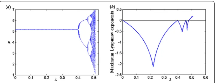
Figure 1(a) Bifurcation diagram of map (1.2) withλ∈(0, 0.55),B= 10,k= 0.95,β= 0.2, the initial value is (5, 5); (b) Maximum Lyapunov exponents corresponding to (a).
In order for map (3.7) to undergo a flip bifurcation, we require that two discriminatory quantitiesα1andα2are not zero, where
α1=
∂2F ∂x˜∂λ∗ +
1 2
δF δλ∗
δ2F δx˜2
(0,0) =h2,
and
α2=
1 6
∂3F ∂x˜3 +
1 2
δ2F δx˜2
2
(0,0)
=h5+h21.
From the above analysis and the theorem of [23], we have the following result.
Theorem 3.1 Ifα2= 0,then map(1.2)undergoes a flip bifurcation at the fixed point(x∗,y∗) when the parameterλ varies in a small neighborhood ofλ1. Moreover, if α2> 0 (resp., α2< 0),then the period-2orbits that bifurcate from(x∗,y∗)are stable(resp.,unstable).
In Sect.4we will give some values of parameters such thatα2= 0; thus, the flip bifurca-tion occurs asλvaries (see Fig.1).
3.2 Neimark–Sacker bifurcation analysis
Finally, we discuss the Neimark–Sacker bifurcation ofE(x∗,y∗) if parameters (B,k,β,λ2) vary in a small neighborhood of HBHB.
Taking parameters (B,k,β,λ2) arbitrarily from HB, we consider system (1.2) with
(B,k,β,λ1), which is described by
⎧ ⎨ ⎩
x→x+λ2x(B x
β
xβ+kyβ –x),
y→y+λ2y(B ky
β
xβ+kyβ –y).
(3.8)
Map (3.8) has a unique positive fixed pointE(x∗,y∗).
Choosingλ∗as a bifurcation parameter, we consider a perturbation of (3.8) as follows:
⎧ ⎨ ⎩
x→x+ (λ2+λ∗)x(B x
β
xβ+kyβ –x),
y→y+ (λ2+λ∗)y(B ky
β
xβ+kyβ –y),
(3.9)
Letu=x–x∗andv=y–y∗. Then we transform the fixed pointE(x∗,y∗) of map (3.9) into the origin. We have
u v
→
a11u+a12v+a13u2+a14uv+a15v2+e1u3+e2u2v+e3v2u+e4v3+O((|u|+|v|)4)
a21u+a22v+a23u2+a24uv+a25v2+d1u3+d2u2v+d3v2u+d4v3+O((|u|+|v|)4)
, (3.10)
wherea11,a12,a13,a14,a15,e1,e2,e3,e4,a21,a22,a23,a24,a25,d1,d2,d3,d4are given in (3.3) by substitutingλforλ2+λ∗.
Note that the characteristic equation associated with the linearization of map (3.10) at (u,v) = (0, 0) is given by
s2+P λ¯∗s+Qλ¯∗= 0,
where
P λ¯∗= –2 –G λ2+λ¯∗
,
Q λ¯∗= 1 +G λ2+λ¯∗
+H λ2+λ¯∗
2 .
Since parameters (B,k,β,λ2)∈HB, the eigenvalues of (0, 0) are a pair of complex conjugate
numberss, and¯swith modulus one by Proposition4, where
s,¯s= –P(λ¯
∗)
2 ±
i 2
4Q λ¯∗–P2 λ¯∗= 1 +(λ2+λ∗)
2 ±
i(λ2+λ∗) 2
√
4H–G2.
Moreover, we have
|s|λ¯∗=0=
Q(0) = 1, l=d|s|
dλ¯∗|λ¯∗=0= – G 2 = 0.
Also, it requires that whenλ¯∗= 0,λm,λ¯m= 1 (m= 1, 2, 3, 4) which is equivalent toP(0)= –2, 0, 1, 2. Note that (B,k,β,λ2)∈HB. Thus,P(0)= –2, 2. We only need to require that
P(0)= 0, 1, which leads to
G2= 2H, 3H. (3.11)
Therefore, the eigenvaluess,¯sof a fixed point (0, 0) of (3.10) do not lie in the intersection of the unit circle with the coordinate axes whenδand (3.11) holds.
Next, we study the normal form of (3.10) atλ¯∗= 0. Letλ¯∗= 0,μ= 1 +Gλ2
2 ,ω= λ2
2
√
4H–G2.
T=
a12 0 μ–a11 –ω
.
Moreover, using the translation
u v
=T
˜
x
˜
y
+e4(μ–a11) –a12d4
In order for system (3.12) to undergo the Neimark–Sacker bifurcation, we require that the following discriminatory quantity is not zero:
a=
From the above analysis, we have the following theorem.
Theorem 3.2 If condition(3.11)holds and a= 0,then map(1.2)undergoes the Neimark– Sacker bifurcation at the fixed point(x∗,y∗)when the parameterλvaries in a small neigh-borhood ofλ2.Moreover,if a< 0 (resp.,a> 0),then an attracting(resp.,repelling)invariant closed curve bifurcates from the fixed point forλ>λ2(resp.,λ<λ2).
4 Numerical simulations
In this section, we illustrate the above analytic results and show the complex dynamical be-haviors by the bifurcation diagrams, phase portraits, and maximum Lyapunov exponents for system (1.2).
For the sake of analysis, we consider the symmetric case of identical firms, letλ1=λ2=λ, β1=β2=β. Then, from system (1.2), we obtain
The bifurcation analyses are considered in the following cases:
(iii) Varyingβin range0.3 <β< 1and fixingk= 0.8,λ= 0.4,B= 10; (iv) Varyingkin range0.35 <k< 2.5and fixingβ= 0.2,λ= 0.4,B= 10.
For case (i). The bifurcation diagram of system (1.2) in the (λ,x) plane for 0 <λ< 0.51 with initial values (x0,y0) = (5, 5) is given in Fig.1(a) to show the dynamical changes asλ varies. The maximum Lyapunov exponents corresponding to the bifurcation diagram in Fig.1(a) are given in Fig.1(b).
In Fig.1, we can see that there is a stable fixed point (5.1602, 4.8398) for 0 <λ< 0.3923, and a flip bifurcation occurs atλ= 0.3923. We observe that there are period-2 orbits for larger regionsλ∈(0.3923, 0.4571).
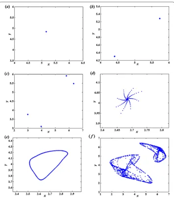
Figure2shows the phase portraits which are associated with Fig.1. Forλ∈(0, 0.55), there are period-1,2,4 orbits (in Fig.2(a)∼(c)). Figure2(d) shows one of the stable fixed points. Figure2(e) shows that the Hopf bifurcations emerge from the fixed points atλ= 0.48. Whenλ= 0.495, we can see the chaotic sets in Fig.2(f ). The maximum Lyapunov
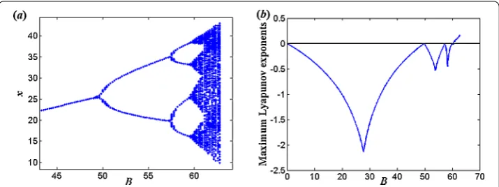
Figure 3(a) Bifurcation diagram of map (1.2) withB∈(0, 62.8),β= 0.2,k= 0.95,λ= 0.08, the initial value is (5, 5); (b) Maximum Lyapunov exponents corresponding to (a).
Figure 4(a) Bifurcation diagram of map (1.2) withβ∈(0, 1),k= 0.8,B= 10,λ= 0.35, the initial value is (5, 5); (b) Maximum Lyapunov exponents corresponding to (a).
exponents corresponding toλ= 0.495 are larger than zero, which confirms the existence of the chaotic sets in Fig.1(b).
For case (ii). The bifurcation diagram of system (1.2) in the (B,x) plane for 0 <B< 62.8 with initial values (x0,y0) = (5, 5) is given in Fig.3(a) to show the dynamical changes asB varies. The maximum Lyapunov exponents corresponding to the bifurcation diagram in Fig.3(a) are given in Fig.3(b).
In Fig.3, a flip bifurcation occurs atB= 49.38 by Proposition1. We observe that there are period-2 orbits for larger regionsB∈(49.38, 57.35). Other cases are similar to case (i). For case (iii). The bifurcation diagram of system (1.2) in the (β,x) plane for 0 <β< 1 with initial values (x0,y0) = (5, 5) is given in Fig.3(a) to show the dynamical changes asβ varies. The maximum Lyapunov exponents corresponding to the bifurcation diagram in Fig.4(a) are given in Fig.4(b).
In Fig.4, we can see that a flip bifurcation occurs atβ= 0.6589 by Proposition1. We observe that there are period-2 orbits for larger regionsβ∈(0.6589, 0.903). Other cases are similar to case (i).
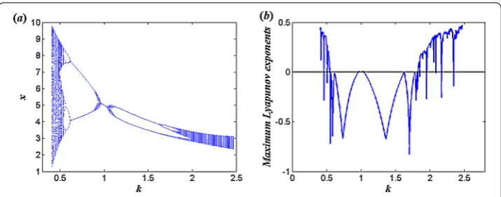
Figure 5(a) Bifurcation diagram of map (1.2) withk∈(0.35, 2.5),β= 0.2,B= 10,λ= 0.4, the initial value is (5, 5); (b) Maximum Lyapunov exponents corresponding to (a).
In Fig.5, there exist double period doubling bifurcations and chaos. We can see that a flip bifurcation occurs atk= 0.9773 ork= 1.027 by Proposition1. We observe that there are period-2 orbits for regionsk∈(0.6261, 0.9773) ork∈(1.027, 1.613). There are period-1, 2, 4, 6, 8, 16 orbits withk= 1, 0.7, 0.58, 1.95, 0.56, 0.55. Whenk= 0.45, 1.9, 2.15, we can see the chaotic sets in Fig.5(a). The maximum Lyapunov exponents corresponding to them are greater than zero, which implies the existence of the chaotic sets in Fig.5(b).
5 Discussion
In this paper, we discuss the dynamical behaviors of model (1.2). From the discussion in Sect.2, we know that there exist flip bifurcation and chaos about equilibrium as the pa-rameters vary in the small neighborhood. We have obtained a global qualitative analysis of model (1.2) depending on all parameters and showed that the model exhibits the bifurca-tions. By choosingλ,B,β,kas bifurcation parameters, respectively, it was shown that the model undergoes a series of bifurcations including the flip bifurcation, period doubling bifurcation, and chaos. Moreover, system (1.2) exhibits many complex dynamic behav-iors, including period-1, 2, 4, 6, 8, 16 orbits, invariant cycle, a cascade of period-doubling, quasi-periodic orbits, and the chaotic sets. These results reveal far richer dynamics of the discrete model compared to the continuous model.
Acknowledgements
The authors thank the anonymous reviewers for their valuable comments.
Funding
This work is supported by the National Natural Science Foundation of China under Grant 61472374, 71503096. China University of Geosciences (Wuhan) Graduate Quality Textbook Construction Project (YJC2017405).
Competing interests
The authors declare that they have no competing interests.
Authors’ contributions
All authors read and approved the final manuscript.
Author details
1School of Education, Minzu University of China, Beijing, P.R. China.2School of Automation, China University of
Geosciences, Wuhan, P.R. China.3Department of Mechanical Engineering, Boston University, Boston, USA.
Publisher’s Note
Springer Nature remains neutral with regard to jurisdictional claims in published maps and institutional affiliations.
References
1. Naert, P., Weverbergh, M.: On the prediction power of market share attraction models. J. Mark. Res.18, 146–153 (1981)
2. Monahan, G.E., Sobel, M.J.: Stochastic dynamic market share attraction games. Games Econ. Behav.6, 130–149 (1994) 3. Bischi, G., Gardini, L., Kopel, M.: Analysis of global bifurcations in a market share attraction model. J. Econ. Dyn. Control
24(5), 855–879 (2000)
4. Kopel, M., Bischi, G.I., Gardini, L.: On new phenomena in dynamic promotional competition models with homogeneous and quasi-homogeneous firms. In: Delli, D.G., Gallegati, M., Kirman, A.P. (eds.) Interaction and Market Structure. Essays on Heterogeneity in Economics, vol. 484, pp. 55–87. Springer, Berlin (2000)
5. Fok, D., Franses, P.H.: Analyzing the effects of a brand introduction on competitive structure using a market share attraction model. Int. J. Res. Mark.21(2), 159–177 (2004)
6. Jing, Z., Jia, Z., Wang, R.: Chaos behavior in the discrete BVP oscillator. Int. J. Bifurc. Chaos12, 619–627 (2002) 7. Jing, Z., Yang, J.P.: Bifurcation and chaos in discrete-time predator-prey system. Chaos Solitons Fractals27, 259–277
(2006)
8. Liu, X., Xiao, D.: Complex dynamic behaviors of a discrete-time predator-prey system. Chaos Solitons Fractals32, 80–94 (2007)
9. Fan, D., Wei, J.: Bifurcation analysis of discrete survival red blood cells model. Commun. Nonlinear Sci. Numer. Simul. 14(8), 3358–3368 (2009)
10. Wang, B., Jian, J.: Stability and Hopf bifurcation analysis on a four-neuron BAM neural network with distributed delays. Commun. Nonlinear Sci. Numer. Simul.15, 189–204 (2010)
11. Shu, H., Wei, J.: Bifurcation analysis in a discrete BAM network model with delays. J. Differ. Equ. Appl.17(1), 69–84 (2011)
12. Hu, Z.Y., Teng, Z., Zhang, L.: Stability and bifurcation analysis of a discrete predator-prey model with nonmonotonic functional response. Nonlinear Anal.12, 2356–2377 (2011)
13. Jiang, X.W., Ding, L., Guan, Z.H., Yuan, F.S.: Bifurcation and chaotic behavior of a discrete-time Ricardo–Malthus model. Nonlinear Dyn.71, 437–446 (2013)
14. He, Z.M., Li, B.O.: Complex dynamic behavior of a discrete-time predator-prey system of Holling-III type. Adv. Differ. Equ.2014, 180 (2014)
15. Xiao, M., Zheng, W., Cao, J.: Stability and bifurcation of genetic regulatory networks with small RNAs and multiple delays. Int. J. Comput. Math.91, 5907–5927 (2014)
16. Ling, G., Guan, Z.H., Liao, R.: Stability and bifurcation analysis of cyclic genetic regulatory networks with mixed time delays. SIAM J. Appl. Dyn. Syst.14(1), 202–220 (2015)
17. Cheng, L., Cao, H.: Bifurcation analysis of a discrete-time ratio-dependent predator-prey model with Allee effect. Commun. Nonlinear Sci. Numer. Simul.38, 288–302 (2016)
18. Yu, P., Lin, W.: Complex dynamics in biological systems arising from multiple limit cycle bifurcation. J. Biol. Dyn.10, 263–285 (2016)
19. Abdelrahman, M.A.E., Chatzarakis, G.E., Li, T., Moaaz, O.: On the difference equationxn+1=axn+bxn–k+f(xn–l;xn–k). Adv.
Differ. Equ.2018, 431 (2018)
20. Wan, X., Wang, Z., Wu, M., Liu, X.:H∞state estimation for discrete-time nonlinear singularly perturbed complex networks under the Round-Robin protocol. IEEE Trans. Neural Netw. Learn. Syst.PP(99), 1–12 (2018) 21. Albert, C.J.L.: Regularity and Complexity in Dynamical Systems. Springer, New York (2012)
22. Guckenheimer, J., Holmes, P.: Nonlinear Oscillations, Dynamical System and Bifurcation of Vector Fields. Springer, New York (1983)
23. Robinson, C.: Dynamical Systems, Stability, Symbolic Dynamics and Chaos, 2nd edn. CRC Press, Boca Raton (1999) 24. Kuznetsov, Y.A.: Elements of Applied Bifurcation Theory, Applied Mathematical Sciences, 3rd edn. Springer, New York
(2004)