One dimensional fractional frequency Fourier transform by inverse difference operator

R E S E A R C H

Open Access

One dimensional fractional frequency

Fourier transform by inverse difference

operator

Dumitru Baleanu

_{, Maysaa Alqurashi}

_{, Meganathan Murugesan}

_and

Britto Antony Xavier Gnanaprakasam

*_{Correspondence:}

[email protected] 1_{Department of Mathematics,} Cankaya University, Ankara, Turkey 2_{Institute of Space Sciences,} Magurele-Bucharest, Romania Full list of author information is available at the end of the article

Abstract

This article aims to develop fractional order convolution theory to bring forth innovative methods for generating fractional Fourier transforms by having recourse to solutions for fractional difference equations. It is evident that fractional difference operators are used to formulate for finding the solutions of problems of distinct physical phenomena. While executing the fractional Fourier transforms, a new technique describing the mechanism of interaction between fractional difference equations and fractional differential equations will be introduced ashtends to zero. Moreover, by employing the theory of discrete fractional Fourier transform of fractional calculus, the modeling techniques will be improved, which would help to construct advanced equipments based on fractional transforms technology using fractional Fourier decomposition method. Numerical examples with graphs are verified and generated by MATLAB.

MSC: 65T50; 39A10; 43A50; 42A38; 42B10; 26A33

Keywords: Fractional Fourier transform; Polynomial factorials; Exponential function; Convolution product; Inverse difference operator and Trigonometric function

1 Introduction

Miller and Ross [27], Oldham and Spanier [29], and Podlubny [31] have developed con-tinuous fractional calculus. The discrete fractional calculus, due to its widespread appli-cations in various branches of science and engineering, has become the object of many research works [1–3,7,14,20]. Recently discrete delta fractional calculus has been devel-oped by Atici and Eloe [12,13,15], Goodrich [21–23], and Holm [24]. For recent develop-ments in the theory of discrete fractional calculus, applications of Mittag-Leffler function and fractional integral inequalities, we refer to [4–6,8,9,16,19,25,26,32].

The integral transforms, like Mellin, Laplace, Fourier, were applied to obtain the so-lution of differential equations. These transforms made effectively possible to change a signal in the time domain into that in the frequency s-domain in the field of Digital Signal Processing (DSP) [34]. The more recent applications of fractional Fourier transform in X-ray models and simulations are developed in [28,30]. In [33], the forward complex DFT,

written in polar form, is given by

be the time between two successive signals. Replacing–1_by–1

, integernby realtand

the sequence x(n) by a functionx(ξ), we get a Generalized Discrete Fourier Transform (GDFT)

The article is organized as follows. InSect.2, the basic concepts about delta and its in-verse difference operators are presented.In Sect.3, one dimensional fractional frequency Fourier transform is defined and its properties with numerical verification are given.In Sect.4, some results on convolution and fractional Fourier transform are discussed. Sec-tion5presents the conclusion.

2 Preliminaries

Here, we present some basic definitions, notations, and preliminaries. Let us denote bysm_r

andSm_r the Stirling numbers of first and second kind, respectively. Denote byR= (–∞,∞),

L(R) = the set of all Lebesgue integrable functions onR. Leth> 0,mbe the positive integer,

νbe a fraction, andωbe the frequency.

The polynomial factorial is defined byt_h(m)=t(t–h)(t– 2h)· · ·(t– (m– 1)h), the relation between the polynomial and polynomial factorials is given by

(i) t_h(m)= fixed shift value. Then theh-difference operatorhonu(t) is defined as follows:

hu(t) =

u(t+h) –u(t)

h , (4)

and its infiniteh-difference sum is defined by

Definition 2.3([17], p. 5, Definition 2.6) Forh> 0 andν∈R, the fallingh-polynomial factorial function is defined by

t_h(ν)=hν Γ( k h+ 1)

Γ(k_h+ 1 –ν), (7)

wherek_h(0)= 1 and k h+ 1,

k

h + 1 –ν∈ {/ 0, –1, –2, –3, . . .}, since the division at a pole yields

zero.

Applying Definition2.1, we get the modified identities as follows:

(i) hth(m)=mt

(m–1)

h , (ii) –1h t

(m)

h =

t(_hm+1) m+ 1,

(iii) –1_h tm=

m

r=1

S_rmhm–rk_h(r) r+ 1 .

(8)

Lemma 2.4 Let h> 0and u(t),w(t)be real-valued bounded functions.Then

–1_h u(t)w(t)=u(t)–1_h w(t) ––1_h –1_h w(t+h)hu(t)

. (9)

Proof Applying (4) on the product of two functionsu(t)v(t), we get

hu(t)v(t) =

u(t+h)v(t+h) –u(t)v(t)

h . (10)

Now the proof follows by adding and subtracting u(t)v_h(t+h), then applying–1_h on both

sides.

Lemma 2.5 Let t∈(–∞,∞),h> 0,andν> 0,then we have

–1_h e–iω1/νt= he

–iω1/νt

(e–iω1/ν_h

– 1). (11)

Proof The proof follows by takingu(t) =e–iω1/νt_{in Definition2.1and applying}–1

h .

Corollary 2.6 Let t∈(–∞,∞),h> 0,andν> 0,then we have

he–iω1/νt

(e–iω1/νh_{– 1)}–

he–iω1/ν(t–mh)

(e–iω1/νh_{– 1)}=h m

r=1

e–iω1/ν(t–rh). (12)

Proof The proof follows by equation (11) and the finite inverse principle law given in (6).

Example2.7 For the particular valuesν= 0.6,s= 0.2,t= 4,m= 2, andh= 3, (12) is verified by MATLAB. The coding is given by 3×symsum(exp(–i×(0.2)(1/0.6)×(4 – 3×r)),r, 1, 2) = (3×exp(–i×(0.2)(1/0.6)_{×4))/(exp(–i×(0.2)}(1/0.6)_{×3) – 1) – (3×exp(–i×(0.2)}(1/0.6)_×

Theorem 2.8 Let t∈(–∞,∞)and h> 0.Then we have

which can be expressed as

–1_h t(2)_h eiω1/νt=

Now (13) follows by continuing the above process and then replacingiby –i.

Theorem 2.9 Let t∈(–∞,∞)and h> 0.If e±iω1/νh_{= 1,then we have}

the proof follows by taking–1_h on both sides.

3 1D fractional frequency Fourier transform and its properties

Definition 3.1 The fractional frequency Fourier transform (FFFT) ofu(t) is defined as follows:

Fh,ν

u(t)=U(ω) =–1_h u(t)e–iω1/νt∞_t=–∞, (16)

and the inverse generalized discrete Fourier transform ofU(s) is given by

u(t) = 1

Similarly, the fractional frequency Fourier sine and cosine transforms ofu(t) are defined as follows:

The inverse of Fourier sine and cosine transforms of the above are respectively given by

u(t) = 2

Letc1andc2be constants. From Definition3.1, we can obtain the following linearity,

change of scale, and shifting properties of fractional frequency Fourier transform.

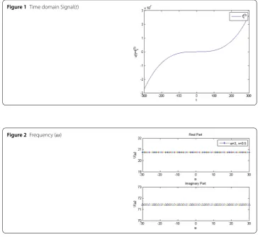
Figure 1Time domain Signal(t)

Figure 2Frequency (ω)

For particular values ofν= 0.5,ω= 3, andh= 1, we provide MATLAB coding for verifi-cation as follows:U(ω) =symsum((4 –r)×(3 –r)×(2 –r)×exp(–i×3(1/0.5)_{×(4 –r)),} r, 1, 8) = (24×(exp(–i×3(1/0.5)_{×4)))/((exp(–i×3}(1/0.5)_{) – 1)) – (36×(exp(–i×3}(1/0.5)_×

5)))/((exp(–i×3(1/0.5)) – 1)2) + (24×(exp(–i×3(1/0.5)×6)))/((exp(–i×3(1/0.5)) – 1)3) – (6× (exp(–i×3(1/0.5)_{×7)))/((exp(–i×3}(1/0.5)_{) – 1)}4_{) + (120×(exp(i×3}(1/0.5)_{×4)))/((exp(–i×}

3(1/0.5)_{) – 1)) + (60×(exp(i×3}(1/0.5)_{×3)))/((exp(–i×3}(1/0.5)_{) – 1)}2_{) + (24×(exp(i×3}(1/0.5)_×

2)))/((exp(–i×3(1/0.5)_{) – 1)}3_{) + (6×(exp(i×3}(1/0.5)_{)))/((exp(–i×3}(1/0.5)_{) – 1)}4_).

The outcomes are generated by MATLAB as diagrams.Figure1is the input function (signal) as polynomial factorial for the time factort.Figure2is the fractional frequency Fourier transform in the frequency domainωfor the particular values ofω= 3 andν= 0.5 which are generated. This shows that the signal runs smoothly in both real and imaginary parts of the frequency domain. One can generate functions easily by varyingωandνto analyze the signal processing in the axis.

4 Convolution product and fractional Fourier transform

In this section, we establish discrete convolution theorem and fractional Fourier transform based on generalized operatorh. Whenh→0, we get convolution theorem and Fourier

Definition 4.1 Letuandvbe two bounded functions on (–∞, +∞). Then the convolution

ofuandvis defined as

w(x) = (u◦v)(x) =–1_h u(t)v(x–t)∞_t=–∞. (27)

It is easy to see thatu◦v=v◦u.

Remark4.2 When bothuandvvanish on the negative real axis,v(x–t) = 0 ift>xand (27) becomes

w(x) = (u◦v)(x) =–1_h u(t)v(x–t)x_t=0. (28)

Theorem 4.3 LetR= (–∞,∞).Assume that u,v∈L(R) =set of all Lebesgue integrable functions onRand that either u or v is bounded onR.Then the convolution

w(x) = (u◦v)(x) =–1_h u(t)v(x–t)∞_–∞ (29)

exists for every x inRand the function w so defined is bounded onR.If,in addition,the bounded function u or v is continuous onR,then w is also continuous onRand w∈L(R).

Proof Sinceu◦v=v◦u, it suffices to consider the case in whichvis bounded. Suppose |v| ≤M. Then

u(t)v(x–t)≤Mu(t). (30)

Sinceu(t)v(x–t) is a measurable function oftonR, from (27) and (30), we get–1 |u(t)×

v(x–t)||∞_–∞≤M–1_h |u(t)||∞_–∞⇒ |w(x)| ≤M–1_h |u(t)||∞_–∞, which tells thatwis bounded onR. Also, ifvis continuous onR, thenwis continuous onR. Now, for every compact interval [a,b], we have

–1_h w(x)b_a≤–1_h u(t)∞_–∞–1_h v(x–t)b_a≤–1_h u(t)∞_–∞–1 v(y)∞_–∞,

wherey=x–t.

Sincewis bounded and continuous onR,w∈L(R).

5 Discrete convolution theorem for discrete Fourier transform

The following theorem illustrates the relation between convolution and Fourier transform.

Theorem 5.1 Assume that u,v∈L(R)and that at least one of u or v is continuous and bounded onR.Let h denote the convolution and w=u◦v.Then,for every realν,we have

–1_h w(x)e–ixν∞ –∞=

–1_h u(t)e–itν∞ –∞

–1_h v(y)e–iyν∞

–∞. (31)

Proof Assume thatvis continuous and bounded onR. Letanandbnbe two increasing

sequences of positive real numbers such thatan→+∞andbn→+∞. Define a sequence

Since|–1

By Lebesgue dominated convergence theorem,

lim

proof. The discrete integral on the left also exists as an improper Riemann integral is con-tinuous and bounded onRand–1_h |w(x)e–ixν_{| ≤}–1

h w|∞–∞for every interval [a,b].

The following example provides the numerical verification of convolution and the solu-tions are analyzed by graphs.

Example5.2 Consider the following functions:

u(t) =

In this work, we proved some properties and results with frequency fractional factorω1/ν

using the inverse difference operator. We defined one dimensional fractional frequency Fourier transform and its convolution. The biggest advantage of our findings is that, when

h→0 andν= 1, the one dimensional fractional frequency Fourier transform becomes the Fourier transform which exists in the literature. We believe that the new extension and definitions will be valuable for researchers to develop the models in Fourier transform. When the Fourier transform does not exist for any function (signal), we can apply one dimensional fractional Fourier transform using (5) and (16) and get several applications in the field of digital signal processing.

Acknowledgements

Funding

Not applicable.

Availability of data and materials

Please contact author for data requests.

Competing interests

All the authors declare that they have no competing interests.

Authors’ contributions

All authors contributed equally and significantly in writing this paper. All the authors read and approved the final manuscript.

Author details

1_{Department of Mathematics, Cankaya University, Ankara, Turkey.}2_{Institute of Space Sciences, Magurele-Bucharest,}

Romania. 3_{Mathematics Department, College of Sciences, King Saud University, Riyadh, Saudi Arabia.}4_{Department of}

Mathematics, Sacred Heart College (Autonomous), Tamilnadu, India.

Publisher’s Note

Springer Nature remains neutral with regard to jurisdictional claims in published maps and institutional affiliations.

Received: 6 November 2018 Accepted: 22 March 2019

References

1. Abdeljawad, T.: Discrete Dyn. Nat. Soc.2013, 406910 (2013) 2. Abdeljawad, T.: Adv. Differ. Equ.2013, 36 (2013)

3. Abdeljawad, T., Atici, F.: Abstr. Appl. Anal.2012, 406757 (2012) 4. Abdeljawad, T., Baleanu, D.: J. Nonlinear Sci. Appl.10, 1098 (2017) 5. Abdeljawad, T., Baleanu, D.: Adv. Differ. Equ.2017, 78 (2017) 6. Abdeljawad, T., Baleanu, D.: Chaos Solitons Fractals102, 106 (2017) 7. Abdeljawad, T., Jarad, F., Baleanu, D.: Adv. Differ. Equ.2012, 72 (2012)

8. Agarwal, P., Al-Mdallal, Q., Cho, Y.J., Jain, S.: Fractional differential equations for the generalized Mittag-Leffler function. Adv. Differ. Equ.2018, 58 (2018)

9. Agarwal, P., El-Sayed, A.A.: Non-standard finite difference and Chebyshev collocation methods for solving fractional diffusion equation. Phys. A, Stat. Mech. Appl.500, 40–49 (2018)

10. Agarwal, R.P.: Difference Equations and Inequalities. Dekker, New York (2000)

11. Akansu, A.N., Poluri, R.: Walsh-like nonlinear phase orthogonal codes for direct sequences CDMA communications. IEEE Trans. Signal Process.55, 3800–3806 (2007)

12. Atici, F.M., Eloe, P.W.: Fractional q-calculus on a time scale. J. Nonlinear Math. Phys.14(3), 333–344 (2007) 13. Atici, F.M., Eloe, P.W.: A transform method in discrete fractional calculus. Int. J. Difference Equ.2(2), 165–176 (2007) 14. Atıcı, F.M., Eloe, P.W.: Electron. J. Qual. Theory Differ. Equ., Spec. Ed. I2009, 1 (2009)

15. Atici, F.M., Eloe, P.W.: Two-point boundary value problems for finite fractional difference equations. J. Differ. Equ. Appl. (2011).https://doi.org/10.1080/10236190903029241

16. Baltaeva, U., Agarwal, P.: Boundary value problems for the third order loaded equation with non characteristic type change boundaries. Math. Methods Appl. Sci.41(9), 3307–3315 (2018)

17. Bastos, N.R.O., Ferreira, R.A.C., Torres, D.F.M.: Discrete-time fractional variational problems. Signal Process.91(3), 513–524 (2011)

18. Britanak, V., Rao, K.R.: The fast generalized discrete Fourier transforms: a unified approach to the discrete sinusoidal transforms computation. Signal Process.79, 135–150 (1999)

19. Choi, J., Agarwal, P.: Certain fractional integral inequalities involving hypergeometric operators. East Asian Math. J. 30(3), 283–291 (2014)

20. Goodrich, C., Peterson, A.: Discrete Fractional Calculus. Springer, New York (2015)

21. Goodrich, C.S.: Solutions to a discrete right-focal boundary value problem. Int. J. Difference Equ.5, 195–216 (2010) 22. Goodrich, C.S.: Continuity of solutions to discrete fractional initial value problems. Comput. Math. Appl.59,

3489–3499 (2010)

23. Goodrich, C.S.: Some new existence results for fractional difference equations. Int. J. Dyn. Syst. Differ. Equ.3, 145–162 (2011)

24. Holm, M.: Sum and difference compositions in discrete fractional calculus. CUBO13(3), 153–184 (2011) 25. Jain, S., Agarwal, P., Kilicman, A.: Pathway fractional integral operator associated with 3m-parametric Mittag-Leffler

functions. Int. J. Appl. Comput. Math.4(5), 115 (2018)

26. Mehrez, K., Agarwal, P.: New Hermite Hadamard type integral inequalities for convex functions and their applications. J. Comput. Appl. Math.350, 274–285 (2018)

27. Miller, K.S., Ross, B.: An Introduction to the Fractional Calculus and Fractional Differential Equations. Wiley, New York (1993)

28. Ni, L., Da, X., Hu, H., Liang, Y., Xu, R.: PHY-aided secure communication via weighted fractional Fourier transform. Wirel. Commun. Mob. Comput.2018, Article ID 7963451 (2018)

29. Oldham, K., Spanier, J.: The Fractional Calculus: Theory and Applications of Differentiation and Integration to Arbitrary Order. Dover, Mineola (2002)

30. Pedersen, A.F., Simons, H., Detlefs, C., Poulsen, H.F.: The fractional Fourier transform as a simulation tool for lens-based X-ray microscopy. J. Synchrotron Radiat.25, 717–728 (2018)

32. Sitho, S., Ntouyas, S.K., Agarwal, P., Tariboon, J.: Noninstantaneous impulsive inequalities via conformable fractional calculus. J. Inequal. Appl.2018, 261 (2018)

33. Smith, J.O.: Mathematics of the Discrete Fourier Transform (DFT). February, 2010 (date accessed), online book 34. Smith, S.W.: The Scientist and Engineer’s Guide to Digital Signal Processing, 2nd edn. California Technical Publishing,