Optimal control in a malaria model: intervention of fumigation and bed nets

(1)

R E S E A R C H

Open Access

Optimal control in a malaria model:

intervention of fumigation and bed nets

Bevina D. Handari

1

_{, Febyan Vitra}

1

_{, Radhiya Ahya}

1

_{, Tengku Nadya S.}

1

_{and Dipo Aldila}

1*

*_{Correspondence:} [email protected] 1_{Department of Mathematics,}

Universitas Indonesia, Depok, Indonesia

Abstract

Malaria is one of the world’s most serious health problems because of the increasing number of cases every year. First, we discuss a deterministic model of epidemic SIR-SI spread of malaria with the intervention of bed nets and fumigation. We found that the malaria-free equilibrium is locally asymptotically stable (LAS) whenR0< 1 and unstable otherwise. A malaria endemic equilibrium exists and is LAS whenR0> 1. Sensitivity analysis ofR0shows that the use of bed nets and fumigation can reduce

R0. We modify the previous model into a stochastic diﬀerential equation model to understand the eﬀect of random environmental factors on the spread of malaria. Numerical simulations show that whenR0> 1, a greater value of noise intensity

σ

generates a solution that is diﬀerent from a deterministic solution; whenR0< 1, regardless of the

σ

value, the solution approaches a deterministic solution. Then the deterministic model was modiﬁed into an optimal control model to determine the best strategy in controlling the spread of malaria by using fumigation as the control variable. Numerical simulations show that periodic fumigations cost less than constant intervention and can reduce the number of infected humans. Priority is given to the endemic prevention strategy rather than to the endemic reduction strategy. For more eﬀective intervention, the value ofR0should receive close attention. A potentially endemic (R0> 1) environment requires more frequent fumigation than an environment that is not potentially endemic (R0< 1). A combination of the use of bed nets and fumigation can reduce the number of infected individuals at minimal cost.

Keywords: Malaria; Optimal control problem; Fumigation; Stochastic diﬀerential equation

1 Introduction

Malaria is a dangerous infectious disease caused by aPlasmodiumparasite, which can be transmitted to humans through bites from infectedAnophelesfemale mosquitos. The symptoms usually appear after one to two weeks and include fever, sweating, shivering or cold, vomiting, headache, diarrhea, and muscle aches (Infodatin [14]). Based on the 2017 World Malaria Report, the number of malaria cases in the world increased to 216 million in 2016. Those cases were mostly located in Africa (90%), Southeast Asia (7%), and the Eastern Mediterranean (2%) (WHO [22]). From 2015 to 2016, malaria cases in Indone-sia reached 217,025 and were mostly found in Papua, Papua Barat, West Nusa Tenggara, Maluku, and North Maluku (Infodatin [14]).

(2)

There are many methods of preventing malaria, the most popular of which are using bed nets at night to prevent mosquito bites and using fumigation to reduce local mosquito populations (WHO [22]). In recent studies, researchers have constructed mathematical models to analyze malaria spread. These include mathematical models of malaria trans-mission that consider climatic factors (Abebe et al. [4]), mathematical models of malaria distribution by using mosquito nets (Agusto et al. [1]; Chitnis et al. [8]; Ngonghala et al. [18]), and mathematical models of climate-based malaria with the use of mosquito nets (Xiunan and Xiao-Qiang [25]), to which this paper refers.

Several factors should be considered when attempting to eliminate malaria vectors, such as climate factors. In tropical areas, there are diﬀerences between mosquito life expectancy in the dry and rainy seasons. Dembele et al. [9] state that there is a greater percentage of deaths from malaria during the rainy season than during the dry season. Therefore this climate factor will be considered in the model.

In this paper, we ﬁrst include two malaria preventatives to the model, the use of bed nets without insecticides and fumigation. First, we construct a deterministic model of the spread of malaria with both fumigation and bed nets. We then determine the equilibrium point and basic reproduction numberR0 followed by numerical simulations to analyze

how both means of intervention aﬀect the human population.

In practice, several factors have been found to aﬀect the spread of malaria, such as hu-man factors (body temperature and carbon dioxide content released by the body) as de-scribed by Keyser [15] and residential factors (living close to stagnant water) as described by Theresa et al. [19]. Both factors are inﬂuenced by unpredictable environmental factors that cannot be explained by the deterministic model. Therefore the deterministic model is extended to a malaria model with stochasticity factors. Next, the stochastic model is discussed by Gray et al. [12], and numerical simulations are implemented to evaluate the dynamics of stochastic factors in spreading malaria throughout the population.

However, some obstacles arose due to the use of fumigation, such as high costs and adverse eﬀects of continuous fumigation on the environment. Hence we ultimately devel-oped the deterministic model into an optimal control problem. Then we analyzed the best strategy for controlling the spread of malaria by using fumigation at minimal cost.

2 Malaria deterministic model with fumigation and bed nets

There are two mathematical models for the spread of malaria in humans: the susceptible infected recovered (SIR) model is used on the human population (h), and the suscepti-ble infected (SI) model is used on theAnophelesmosquito population (v). The diﬀerence between the two models lies in the recovered (R) compartment, which only humans pos-sess;Anophelesmosquitos’ lifespans are too short for them to enter this stage. Both human and mosquito populations were assumed to be homogeneous closed populations; thus the total populations of humansNhand mosquitosNvcan be considered to be the sums of

(3)

only in a short time period with considering a short time period of intervention. Therefore we put aside the death rate due to malaria from our model. With this assumption, we have that all human deaths are considered natural. Fumigation and the use of bed nets were used in the models as means of intervention to eliminate malaria with the assumption that no mosquitos are resistant to fumigation. Note that the long-term intervention of fu-migation may lead to genetic mutation of mosquitoes as described by Bustamam, Aldila, and Yuwanda [6].

The malaria infection process is assumed to happen with successful infection probabil-itieschandcvand with mosquito bite rates ofβhandβv. The use of bed nets can decrease

the total number of mosquito bites. However, since not all people use bed nets at home, the mosquito bite rate is deﬁned as follows:

βi(k,η) =βikη+βi(1 –k),

wherekindicates the proportion of humans who use bed net, andηindicates the eﬀec-tiveness of the bed nets. An increase inkindicates the increasing number of people using bed nets. On the other hand, an increase inηresults in poorer prevention of mosquito bites related to the quality of the bed nets. Note thatηandkare bounded parameters in [0, 1]. Human and mosquito deaths in the model are only caused by natural deathsμhand μv, respectively, although mosquito deaths are also caused by fumigationu.

The recovery rate of humans isγ and can revert to being susceptible at rateδ. The ﬂow diagram model is seen in Fig.1.

According to Fig.1, the SIR-SI mathematical model of malaria disease spread with fu-migation and bed nets is as follows:

dSh

dt =Ah–

chβh(k,η)ShIv

Nh

–μhSh+δRh,

dIh

dt =

chβh(k,η)ShIv

Nh

–γIh–μhIh,

(4)

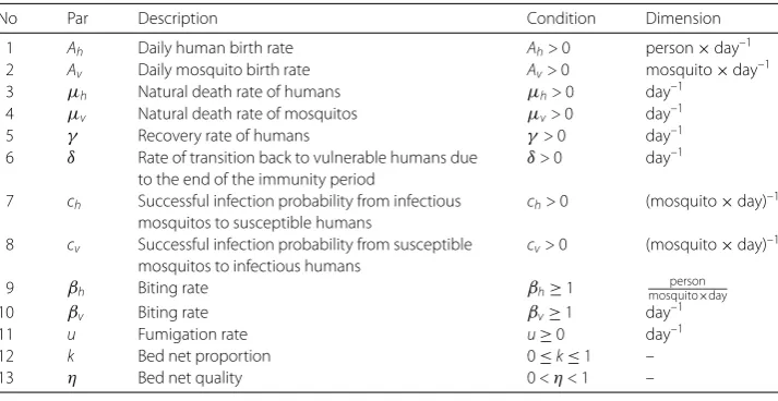
Table 1 Parameters of SIR-SI model (1)

No Par Description Condition Dimension

1 Ah Daily human birth rate Ah> 0 person×day–1

2 Av Daily mosquito birth rate Av> 0 mosquito×day–1

3 μh Natural death rate of humans μh> 0 day–1

4 μv Natural death rate of mosquitos μv> 0 day–1

5 γ Recovery rate of humans γ> 0 day–1

6 δ Rate of transition back to vulnerable humans due to the end of the immunity period

δ> 0 day–1

7 ch Successful infection probability from infectious

mosquitos to susceptible humans

ch> 0 (mosquito×day)–1

8 cv Successful infection probability from susceptible

mosquitos to infectious humans

whereμv(t) andu(t) are functions depending on time, which describe seasonality and

fu-migation in mosquito population, respectively. Later we will discuss further details about the dependency of these parameter on time. For the analysis of model (1) related to their equilibrium point and their basic reproduction number, we assume that u(t) =u and μv(t) =μvas constant parameters. The description of parameters in model (1) is given

in Table1. Since we assume that without fumigation intervention, the total human and mosquito populations are constant, we have that

d(Sh+Ih+Rh)

which indicates that the total number of mosquitoes decreases with respect to time. Next, we analyze the equilibrium points and the corresponding basic reproduction num-berR0. The equilibrium points of the model are the malaria-free equilibrium (MFE) and

(5)

MFE represents a condition where no individual is infected with malaria. Furthermore,

MFE has positive values onR+

5, which means that it always exists biologically. (a) The basic reproduction numberR0is used to analyze whether the malaria is

endemic (R0≥1) or not (R0< 1).R0can be constructed using the next-generation matrix (NGM) method [10]. Please see [2,3,6] for further examples of the

construction of the NGM for epidemic models. First, we construct the Jacobian matrix of infected compartments constructed from system (1):

J=

The matrixJis decomposed into a transmission matrixT that contains the infectious parameter and a transition matrixVthat does not contain the infectious parameter as follows:

Therefore NGM is written as

NGM= –TV–1=

andR0is the spectral radius of NGM,

R0=

u+μv. Further discussion aboutR0will be given later in this

section.

(b) MEE represents a condition in which malaria always persists in a population. The MEE of the model is as follows:

(6)

with

(c) The stability of the two equilibrium points can be determined with eigenvalue analysis from a system evaluated at the corresponding equilibrium point. To determine the stability of MFE, system (1) must be linearized on MFE as follows:

JDFE=

where the characteristic polynomial of (6) is

(λ+δ+μh)(λ+μh)(λ+u+μv)

Next, we analyze the stability of the MEE point. Substituting the MEE into the Jacobian matrix of system (1), we obtain ﬁve eigenvalues, with two of themλ1= –(μv+u) andλ2=

–μh. The other three eigenvalues are taken from the root of the third-degree polynomial

given by

(7)

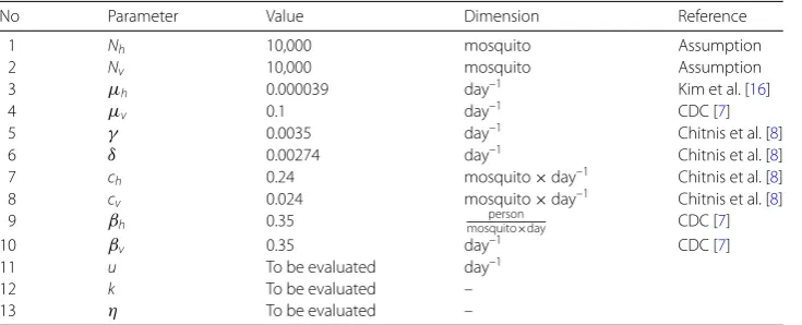
Table 2 Parameter values of SIR-SI model (1)

No Parameter Value Dimension Reference

1 Nh 10,000 mosquito Assumption

2 Nv 10,000 mosquito Assumption

3 μh 0.000039 day–1 Kim et al. [16]

to the Routh–Hurwitz stability criteria, all roots of (8) are negative ifa2> 0,a0> 0, and

a2a1>a0. Therefore we have that the MEE of system (1) is locally asymptotically stable if

R0> 1 anda2a1>a0. On the other hand, whenR0< 1 ora2a1≤a0, the MEE is unstable.

To understand the role of model parameters to the basic reproduction numberR0, we

analyze the sensitivity ofR0and perform autonomous simulation of the given intervention

parameter. According to Kim et al. [16], both simulations use the initial conditionsSh(0) =

0.5148Nh,Ih(0) = 0.2113Nh,Rh(0) =Nh–Sh(0) –Ih(0),Sv(0) =Nv–Iv(0),Iv(0) = 0.3267Nv,

and the parameter values used are listed in Table2.

Sensitivity analysis ofR0is implemented because it is related to policies that might be

used by related parties. The ﬁrst analysis is theR0sensitivity of the mosquito biting rate

toward humans,βh(k,η) withk= 0, and without the use of bed nets. The second analysis

isR0sensitivity toward the fumigation rateu. An analytical study onR0can be obtained

as follows:

Equation (9a) is always positive, which means that the curve of the biting rate parame-ter towardR0is increasing monotonically, or asβhincreases,R0also increases. On the

other hand, Eq. (9b) is always negative, which means that the curve of the fumigation rate parameter towardR0is decreasing monotonically, or asuincreases,R0decreases.

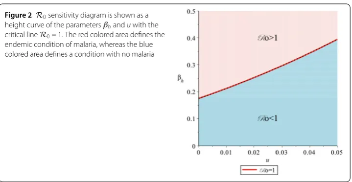
When we substitute all parameters value from Table 2 into R0 = 1, we have 0.238673939√β_h

u+0.1 = 1. Figure 2 explains how R0 can be determined by relying on u and

βh qualitatively based on the previous equation. It can be seen from Fig.2 that when

βh< 0.17554563, the population always achieves a malaria-free situation (R0< 1), and

thus fumigation is not yet needed. Whenβh> 0.175545635, fumigation is needed to reach R0< 1. By solving

0.238673939√βh

u+0.1 = 1 with respect touwe have

(8)

Figure 2 R0sensitivity diagram is shown as a height curve of the parametersβhanduwith the

critical lineR0= 1. The red colored area deﬁnes the endemic condition of malaria, whereas the blue colored area deﬁnes a condition with no malaria

Therefore, when βh > 0.175545635, we needu>umin to achieve the conditionR0< 1.

This study indicates that there is a possibility that fumigation is not needed to eliminate malaria from humans. It is shown through the above simulation that when the infection rate is lower than the minimum boundary ofuthat yieldsR0< 1, fumigation is not needed.

Furthermore, there are other parameters to consider when fumigation should be imple-mented in the ﬁeld to yieldR0< 1, which is an infection rate.

The second analysis isR0sensitivity toward the bed net parameter, which is the

pro-portion of the userskand the proportion of bed net eﬀectivenessη. The analytical study onR0is as follows:

∂R0

∂k = –

chβhcvβv(1 –η)2Nv

(γ+μv)(u+μv)Nh

, (11a)

∂R0

∂η =

chβhcvβvkNv

(γ+μv)(u+μv)Nh

. (11b)

According to Table1, the parameterηis in the interval (0, 1), andkis in the interval [0, 1]; thus we can guarantee that (η– 1) < 0 and (1 –k)≥0. This means that Eq. (11a) shows thatR0decreases monotonically with respect tok; that is, askincreases,R0

de-creases. Equation (11b) shows thatR0monotonically increases with respect toη; thus, as

ηincreases,R0also increases.

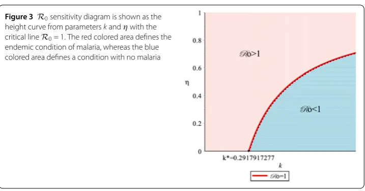
Using the same approach as in Fig.2, we substitute all parameters values from Table2 exceptkandη, which gives us 4.034325733(0.35(kη–k+ 1))2_{= 1. Figure}₃_{explains how}

R0can be determined by relying onkandηqualitatively. Figure3also further elucidates

the threshold ofR0; the red colored area deﬁnes a condition withR0> 1, and the blue

colored area deﬁnes a condition withR0< 1.

It can be seen in Fig.3that whenk≤k∗= 0.2917917277, the bed net usage intervention does not eliminate malaria; thus the proportion of bed net users must endeavor to achieve

(9)

Figure 3 R0sensitivity diagram is shown as the height curve from parameterskandηwith the critical lineR0= 1. The red colored area deﬁnes the endemic condition of malaria, whereas the blue colored area deﬁnes a condition with no malaria

the bed nets is important to achieveR0< 1. Solving 4.034325733

(0.35(kη–k+ 1))2_{= 1}

with respect toη, we have

ηmin=

k– 0.2917917277

k . (12)

Therefore, whenk>k∗, we needη>ηminto achieve the conditionR0< 1. This means that

when providing bed nets, the quality of the bed nets needs to be considered. The better the quality of the bed nets, the higher the chance that the bed nets decrease the number of mosquito bites; thus the proportion of bed net use is lower whenkk∗.

The life expectancy of mosquitos is different during the rainy season than in the dry one, making their natural death rates different as well. The natural death rate depends on time orμv(t). For example, the rainy season happens in the first six months followed by

the dry season in the next six months on the interval [0, 365]. Assuming that the natural death of mosquitos in the dry season is twice that in the rainy season, the natural death of mosquitos can be formulated as follows:

μv(t)

⎧ ⎨ ⎩

μ1= 0.1, 0 <t<365₂ ,

μ2= 0.2, 365₂ <t< 365,

(13)

whereμ1is the natural death rate of the mosquito during the rainy season, andμ2is the

natural death rate during the dry season. In real circumstances, there is a transition season between both seasons. Therefore Eq. (13) needs to be changed into a continuous function by using a Fourier series (Wrede and Spiegel [24]). By including the transition season the natural death rate of mosquitos can be stated as follows:

μv(t) = 0.15 – 0.06366197724sin

2 365πt

– 0.02122065908sin

6 365πt

. (14)

(10)

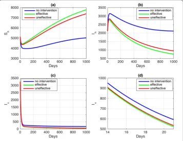
selected; in other words, the fumigation rate in the rainy season is higher than the rate during the dry season. Next, to compare the impacts of different types of fumigation, we performed an autonomous simulation for compartment models with differences in the fu-migation parameteru. The simulation excludes the bed net intervention (k= 0). The first fumigation parameter has a constant fumigation rateu= 0.05. The second fumigation rate is given periodically on the first day of the month by considering the season in Eq. (13) for 720 days, and the fumigation rates during the dry and rainy seasons areu1= 1 andu2= 2, respectively. The simulation does not include fumigation.

Fumigation is expected to suppress the mosquito populations so that there will be no vectors that can spread malaria. In Fig.4, there is a quite a significant difference in the curves with fumigation compared to the curve without fumigation. Since no fumigation is implemented (blue curve), the number of susceptible humans decreased, which is caused by the high intensity of infections and is confirmed by the increased numbers of infected humans. On the other hand, the natural number of mosquitos decreases with or with-out fumigation. However, the implementation of fumigation accelerates the decrease of infected mosquitos and suppresses the endemic point. The plot on the bottom right of Fig.4shows the differences between no intervention, constant fumigation, and two sea-sons fumigation and shows a significant drop in the green curve due to a difference in the fumigation rates. With seasons, the total population of the mosquito tends to zero with

R0= 0.9413426708 < 1, and the epidemic eventually disappears. However, with no

inter-vention, the value ofR0becomesR0= 1.412014006 > 1; in other words, the endemic state

still exists.

(11)

Figure 5Autonomous simulations with changes in parameterk. The blue curve represents no intervention, the red curve indicates that the bed nets are not eﬀective, and the green curve indicates that the bed nets are eﬀective

The use of bed nets in endemic areas is expected to be able to prevent the spread of malaria through mosquito bites. In this simulation, to suppress the number of infected people, we choose a situation where no fumigation is performed (u= 0). The autonomous simulation of bed nets is shown in Fig.5.

In Fig.5, when the bed nets are used, the blue curve shows that malaria persists with

R0= 1.412014007 > 1. The red curve describes a population with bed nets but without

taking into account the minimum qualityηof the bed nets, resulting in ineﬀectiveness withR0= 1.059010505 > 1. However, if the value ofηis chosen based on the previousR0

sensitivity (η= 0.4), then, as seen in the green curve, the population is freed from malaria withR0= 0.9884098046 < 1. Although the diﬀerence inR0is not signiﬁcant, overall, we

can state that not only should the proportionkof bed nets usage be considered, but also the qualityηof the bed nets should be considered. Note that bed nets are given to prevent mosquitos from biting humans, not to reduce the number of mosquitos. Therefore the diﬀerence in each scenario in the mosquito population is not signiﬁcant.

3 Malaria model with environment stochasticity

In the previous sections, we used a deterministic model of malaria spread where all pa-rameters are constant. In real-world conditions, there are environmental factors that are crucial to the spread of malaria, such as body temperature, CO2 levels released by

(12)

Since the above environmental factors are related to the inﬂuence of the mosquito biting

increment of a Brownian motion (Higham [13]).

By substituting Eqs. (15) into the deterministic model (1) we obtain the following SDEs:

dSh=

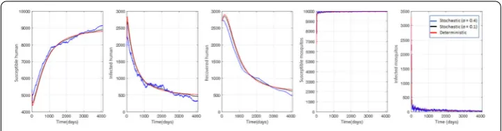
Next, we performed numerical simulations to determine the eﬀects of stochastic factors and the implications of parameter changes on the SDE model (16). Simulations were per-formed for as many as 250 iterations using the Euler–Maruyama method for 4096 days with two scenarios, a simulation of fumigation intervention and a simulation of bed net intervention. In the following simulation results, the ﬁrst three curves are for human pop-ulations, and the last two curves are for mosquito populations.

Simulations of fumigation are divided into two cases, cases without (Figs.6–7) and with (Fig.8) time-dependent mosquito death rates. Since the simulations focus on fumigation, we set the parameter of the bed net proportion tok= 0. Based on Eq. (10), the fumigation rateu= 0.02 is selected forR0> 1, andu= 0.06 forR0< 1. Figure6shows the conditions

for endemic disease (R0> 1). The stochastic trends are quite diﬀerent from the

determin-istic trends. The greater the value of noise intensityσ, the more significant the fluctuations in the simulations, which means that when an epidemic occurs, the greater environmen-tal factors significantly affect the dynamics of all subpopulations. The results in Fig.7are quite different from those in Fig.6, where the stochastic trend is approaching a determin-istic trend. The noise intensity value does not significantly affect the fluctuations. In other words, whenR0< 1, environmental factors will not significantly affect the dynamics of

the subpopulations. These situations appear because the environment stochasticity is in-cluded in the infection term (βi) in our model. WhenR0> 1, infected compartments tend

toward nonzero equilibrium, which makes it easy to capture the impact ofσ. On the other hand, whenR0< 1, where all infected compartments tend toward the zero-equilibrium

point, the impact ofσ is lower, and all variables signiﬁcantly ﬂuctuate.

For the second case, we consider the inﬂuence of the season on the mosquito death rate μvsince the life expectancy of mosquitos during rainy and dry season is variable. A

(13)

Figure 6Model simulation with fumigation and without bed nets whenR0> 1

Figure 7Model simulation with fumigation and without bed nets whenR0< 1

Figure 8Model simulation with periodic fumigations and without bed nets with the inﬂuence of the season

is given on the ﬁrst day of the month periodically for 720 days. In Fig.8, the curves from susceptible mosquitos and infected mosquitos oscillate every 30 days due to the season and periodic fumigation. The dynamics of the human population also cause oscillations with smaller ﬂuctuations than those of the mosquito population because the dynamics of the mosquito population dynamics gain stability more quickly than those of the human population. We refer to this situation as a fast dynamics and slow dynamics for mosquitos and humans, respectively, which means that when an epidemic of malaria occurs, the more random the environment, the more unpredictable the dynamics of malaria over a short-term period.

Analyzing the eﬀects of bed net intervention, we set the fumigation parameteruequal to 0. Based on Eq. (12), the proportion of bed nets isk= 0.5, and the eﬀectiveness of bed nets isη= 0.5 forR0> 1, whereasη= 0.4 forR0< 1. The results in Figs.9and10are

(14)

Figure 9Model simulation with bed netsη= 0.5 and without fumigation whenR0> 1

Figure 10 Model simulation with bed netsη= 0.4 and without fumigation whenR0< 1

Figure 11 Model simulation with fumigation and without bed nets whenR0> 1

Note that all above simulations result from one of the stochastic simulations. Of interest is that the mean of the 250 stochastic simulations shows a diﬀerent performance. For ex-ample, in the simulation in Fig.11the mean solution is quite similar to the deterministic solution. In other words, the mean curve of the stochastic simulations is close to that of the deterministic model. The same results also have been mentioned in previous studies (Feng et al. [11]; Banks, Catenacci and Hu [5]). Simulations using other scenarios also have the same characteristics as simulations in Fig.11.

4 Optimal control problem

There are several obstacles in using fumigation. One of these is the high cost of fumigation. To overcome this problem, the deterministic model (1) can be developed into an optimal control problem where the fumigation parameteru, which was previously set as a con-stant, now changes into a control variableu(t) that depends on time. The purpose of this optimal control problem is determining the continuous piecewise function of the control variableu(t) in the intervalt0= 0 throught1=T, which reduces infected populations at a

minimum cost.

We assume the costs to reduce the numbers of infected individuals with malariaIh(t) and

(15)

proportional to the numbers of infected humans and mosquitos. However, the cost of fumigation is a nonlinear function because a wider area of intervention causes a sharp, nonlinear cost increase. Therefore the objective function of the spread of malaria with fumigation can be written as follows:

Ju(t)=

minimize the number of infected individuals, we setω2andω5greater than 0, whereas the

other parameters are set to 0. Since higher numbers of fumigations elevate the intervention cost, we setωv> 0. Therefore we have

We assume that the controlu(t) is not carried out all the time; instead, it is periodically used everyhdays forTdays. Thereforeu(t) can be represented as a semidiscrete function (Wijaya et al. [21]) is the value of the control variable at timetgiven in Eq. (21).

Next, we deﬁne the Hamiltonian (Lenhart et al. [17]). The Hamiltonian consists of the sum of the integrand of the objective function in Eq. (17) and the inner products of the state in Eq. (1) with the adjoint variableλk,k= 1, 2, 3, 4, 5. The Hamiltonian H(xi,u,λk) can

Theorem 1 Given an optimal control variable u(t)that minimizes objective function J

(16)

variables

with the transversality condition for adjoint variables

λk(t) = 0, k= 1, 2, 3, 4, 5.

Since the admissible control should be bounded with uminand umaxas the lower and upper bounds of u(t),respectively,the control variable u(t)is represented by

ˆ

Proof We ﬁrst diﬀerentiate the negative of the Hamiltonian (19) with respect to each state variable, so the adjoint variables have the following form:

˙

with the transversality condition for adjoint variables

λk(T) = 0, k= 1, 2, 3, 4, 5.

To obtain optimal conditions, we also diﬀerentiate the Hamiltonian (19) with respect to

u(t) and set these equations equal to zero:

∂H ∂u(t)= 2ωu

(17)

Solving (22) with respect to the control variable, we obtain

u∗(t) =λ4Sv(t) +λ5Iv(t) 2ωu

. (23)

The control variableu∗(t) in (23) must satisfyumin≤u∗(t)≤umaxfor allt∈[0,T], and then the control variableuˆ(t) can be written as

ˆ

u(t) =min

umax,max

umin,λ4Sv(t) +λ5Iv(t) 2ωu(t)

,

where umax andumin are the lower and upper bounds for the control variable,

respec-tively.

Several scenarios are implemented in numerical simulations based on the results of The-orem1. The simulations are conducted using four different scenarios, that is, different val-ues ofR0(e.g., seasonal influence, implementation of bed nets, and different initial

con-ditions). To ﬁnd a balance between each component in the cost function (17), we choose ω2= 0.5,ω5= 0.0025, andωu= 0.01. Note that our control variable is a rate of

interven-tion, which can tend to∞. Therefore we can choose the interval value of fumigation is 0≤u(t)≤5 with the time interval of 0≤t≤500 days. Fumigations are conducted peri-odically every 30 days for 500 days. It is assumed that one intervention will have an impact for the next three days. In numerical simulations we used the iterative gradient descent algorithm to accelerate the convergence of the control variableu(t).

Numerical simulations are conducted with and without fumigation when R0 > 1

andR0< 1 and for the purpose of comparing the reductions of infected humans and

mosquitos. TheR0 formula refers to Eq. (6). The initial values of each population are Sh(0) = 8000,Ih(0) = 1900,Rh(0) = 100,Sv(0) = 8000, andIv(0) = 2000.

Based on the results in Fig. 2, the biting rate value of mosquitos must satisfy βh <

0.17554563 to satisfyR0< 1; thus we choose the parameter valuesβh=βv= 0.17, which

givesR0= 0.6868. On the other hand, in the case whereR0> 1, which describes an

epi-demic that still exists in the environment, we have chosen the value forβh=βv= 0.35,

which gives the result forR0= 1.412.

Figure12shows changes in the number of infected humans and mosquitos for 500 days. The dynamics of the control variablesu(t) in the cases ofR0> 1 andR0< 1 have similar

behavior; that is, when infected mosquitos exist, fumigation must be performed. However, when the number of infected mosquitos begins to decrease, the intervention must be re-duced. The intervention in the case ofR0< 1 decreases faster due to rapidly reduced

num-bers of infected mosquitos compared to the case ofR0> 1. As a result, the cost function

ofR0> 1 is 3.4632225×105, whereas in the case ofR0< 1, it is only 2.535228×105. This

result appears because, under the conditionR0< 1, the environment most likely tends to

a malaria-free equilibrium even though fumigation is not implemented. However, this fu-migation policy faster achieves the malaria-free equilibrium. Therefore, the cost function whenR0< 1 is much lower than whenR0> 1.

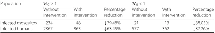
In Table3, in the cases ofR0> 1 andR0< 1, fumigation is equally successful in reducing

the number of infected mosquito populations. In the case ofR0> 1 the reduction in the

(18)

Figure 12 Numerical simulations in the cases ofR0> 1 andR0< 1

Table 3 Number of infected individuals on day 500 in the cases ofR₀< 1 andR₀> 1

Population R0> 1 R0< 1

Without intervention

With intervention

Percentage reduction

With intervention

Infected mosquitos 234 48 ↓79.48% 21 13 ↓38.05%

Infected humans 2367 865 ↓63.45% 577 362 ↓37.26%

in the case of R0< 1, it was 38.05%. The results are similar for the number of infected

humans.

In the following simulations, we aim to determine the dynamics for infected humans and mosquitos with and without fumigation by seasonal and nonseasonal inﬂuence. As in Sect.2, the mosquito mortality rateμv, which was constant, is converted into a function

as in Eq. (14).

Based on Figs.13and14, a fumigation intervention is successful in reducing the num-ber of infected humans and mosquitos, and the numnum-ber of reductions is shown in Table4. However, when the seasonal influence is considered, the intervention effects decrease sig-nificantly when the rainy season period ends (t= 182). The cost function when there is a seasonal influence is 3.3577×105_{, whereas when there is no seasonal influence, it is}

3.4632225×105.

(19)

Figure 13 Numerical simulation results with and without fumigation in cases of nonseasonal inﬂuence

(20)

Table 4 Number of humans and mosquitos infected on day 500 with seasonal inﬂuence

Populations R0> 1 R0< 1

With intervention

Infected humans 1905 803 ↓57.84% 2367 923 ↓61.00%

Figure 15 Results of simulations with and without fumigation intervention whenk= 0 andk= 0.2

case is where there are no people using bed nets (k= 0), and in the second case, 20% of the total population uses bed nets (k= 0.2).

Changes in the number of infected humans and mosquitos and the dynamics of the con-trol variableu(t) can be seen in Fig.15. The dynamics of the control variables show similar behavior in both cases. However, the fumigation used for casek= 0 is greater than the in-tervention in the case ofk= 0.2. The cost function for the case ofk= 0 is 3.46322×105

compared to that for the case ofk= 0.2, which is 3.73323×105. Therefore the combina-tion of bed nets and fumigacombina-tion can reduce the number of infected mosquitos and humans with minimal cost compared to the numbers from the case without the combination.

(21)

Table 5 The number of infected individuals on day 500 whenk= 0 andk= 0.2

Population k= 0 k= 0.2

With intervention

Infected humans 1905 803 ↓57.84% 1659 627 ↓62.2%

Figure 16 Numerical simulation results with and without fumigation in the endemic reduction scenario

Finally, we want to understand the influence of fumigation under two conditions that ex-ist in the human population, endemic reduction and endemic prevention. The difference between the two conditions is the number of mosquitos and humans infected at the initial conditiont= 0, where in the endemic reduction scenario the number of infected individu-als is relatively high as compared to the endemic prevention condition. Here we use initial conditions to illustrate the possible situations that occur in the field. In the endemic re-duction scenario the initial values areSh(0) = 8000,Ih(0) = 1900,Rh(0) = 100,Sv(0) = 8000,

andIv(0) = 2000. In the endemic prevention scenario, the initial values areSh(0) = 9900,

Ih(0) = 80,Rh(0) = 20,Sv(0) = 9950, andIv(0) = 50.

The endemic reduction scenario illustrates cases that occur in the ﬁeld when malaria infection has spread. The number of infected individuals (humans and mosquitos) and the dynamics of the control variableu(t) are shown in Fig.16. Table6shows the reduction in the number of infected individuals for this scenario after a period of time.

(22)

Table 6 The numbers of each population of infected individuals on the 500th day of the endemic reduction scenario

Population Without

intervention With intervention

Infected mosquitos 168 45 ↓73.21%

Infected humans 1905 803 _↓57.84%

Figure 17 Numerical simulation results with and without fumigation in the endemic prevention scenario

Table 7 The number of each population of infected individuals on the 500th day of the endemic prevention scenario

Population Without

intervention With intervention

Infected mosquitos 35 5 ↓85.71%

Infected humans 434 59 ↓86.41%

in Fig.17. Table7contains information on the reduction numbers for infected individuals at the 500th day.

(23)

better if it is performed during the early stages of the endemic. Therefore an early warning system for malaria endemics should be considered to achieve better malaria prevention results.

Tables6and7show that the percentage reduction of the endemic prevention scenario is larger than that of the endemic reduction scenario. This is because the number of in-fected individuals to be reduced in an endemic reduction scenario is greater than that in an endemic prevention scenario.

5 Conclusion

The deterministic model of epidemic spread of malaria with bed nets and fumigation interventions has a malaria-free equilibrium (MFE), which always exists biologically, whereas the malaria endemic equilibrium (MEE) exists whenR0> 1. The MFE is

asymp-totically stable whenR0< 1, whereas MEE can be stated as a stable point under the

con-ditionR0≥1. The simulation results show that fumigation is not needed when the

in-fection rate is less than the minimum boundary of the fumigation rate such thatR0< 1.

In bed net interventions, when the proportion of bed nets used is less than the minimum value, bed nets will not eliminate malaria; thus the proportion of bed net users needs to be evaluated. Additionally, the better the quality of the bed nets, the higher the chance of reducing the number of mosquito bites. Simulations also show that when fumigation is not performed, many healthy humans become infected. Additionally, fumigation needs to be adjusted depending on season. By incorporating the seasonal inﬂuence the popula-tion of mosquitos reduces withR0= 0.9413426708 < 1. However, with no intervention,

R0= 1.412014006 > 1; in other words, the malaria epidemic will still exist.

To observe the effect of random environmental factors on the spread of malaria, we considered a stochastic model. Numerical simulations were performed to determine the effects of stochastic factors and the implications of parameter changes on the model. The simulations show that when an epidemic exists, the environmental factors significantly affect the dynamics within all subpopulations. However, whenR0< 1, the environmental

factors do not greatly aﬀect the dynamics of the subpopulations.

When the intervention is performed every 30 days, the numbers of susceptible and in-fected mosquitos oscillate every 30 days due to the inﬂuence of the season and fumigation. Reducing the infected population requires using smaller values for the eﬀectiveness of bed nets. These results are consistent with the analytic solution in the deterministic case.

(24)

was also investigated. Fumigation has successfully reduced the numbers of infected hu-mans and mosquitos. The dynamic control variable shows that if the number of infected mosquitos increases, then fumigation is required; on the other hand, fumigation must be performed less frequently if there are fewer infected mosquitos. The cost function for the endemic reduction scenario is higher than the cost function for the endemic prevention scenario.

Funding

This research was ﬁnancially supported by the Indonesia Ministry of Research and Higher Education (Kemenristek DIKTI) with PUPT research grant scheme 2018 with project ID No. 367/UN2.R3.1/HKP05.00/2018.

Competing interests

The authors declare that they have no competing interests.

Authors’ contributions

All authors carried out the proofs of the main results and approved the ﬁnal manuscript.

Publisher’s Note

Springer Nature remains neutral with regard to jurisdictional claims in published maps and institutional aﬃliations.

Received: 10 December 2018 Accepted: 18 November 2019 References

1. Agusto, F.B., Valle, S.Y., Blayneh, K.W., et al.: The impact of bed-net use on malaria prevalence. J. Theor. Biol.320, 58–65 (2013)

2. Aldila, D., Nuraini, N., Soewono, E.: Mathematical model in controlling dengue transmission with sterile mosquito strategies. AIP Conf. Proc.1677, 030002 (2015)

3. Aldila, D., Padma, H., Khotimah, K., Handari, B.D., Tasman, H.: Analyzing the MERS control strategy through an optimal control problem. Int. J. Appl. Math. Comput. Sci.28(1), 169–184 (2018)

4. Alemu, A., Abebe, G., Tsegaye, W., Golassa, L.: Climatic variables and malaria transmission dynamics in Jimma town, South West Ethiopia. Parasites Vectors4(1), Article ID 30 (2011)

5. Banks, H.T., Catenacci, J., Hu, S.: A comparison of stochastic systems with diﬀerent types of delays. Stoch. Anal. Appl. 31(6), 913–955 (2013)

6. Bustamam, A., Aldila, D., Yuwanda, A.: Understanding dengue control for short and long term intervention with a mathematical model approach. J. Appl. Math.2018, Article ID 9674138 (2018)

7. CDC:Anophelesmosquitos. Centers for Disease Control and Prevention (2015)

8. Chitnis, N., Hardy, D., Gnaegi, G., et al.: Modeling the eﬀects of vector control interventions in reducing malaria transmission, morbidity and mortality. Malar. J.9(Suppl 2), Article ID O7 (2010)

9. Dembele, B., Friedman, A., Yakubu, A.: Malaria model with periodic mosquito birth and death rates. J. Biol. Dyn.3(4), 430–445 (2009)

10. Diekmann, O., Heesterbeek, J.A.P.: Mathematical Epidemiology of Infectious Diseases: Model Building, Analysis and Interpretation. Wiley, New York (2000)

11. Feng, Z., Liu, R., Qiu, Z., Rivera, J., Yakubu, A.: Coexistence of competitors in deterministic and stochastic patchy environments. J. Biol. Dyn.5(5), 454–473 (2011)

12. Gray, A., Greenhalgh, D., Hu, L., Mao, X., Pan, J.: A stochastic diﬀerential equation SIS epidemic model. SIAM J. Appl. Math.71(3), 876–902 (2011)

13. Higham, D.J.: An algorithmic introduction to numerical simulation of stochastic diﬀerential equation. SIAM Rev.43(3), 525–546 (2001)

14. Infodatin: Malaria. InfoDATIN (Pusat Data dan Informasi Kementerian Kesehatan RI). Kementerian Kesehatan RI, Jakarta (2016)

15. Keyser, H.: Why are some people more prone to mosquito bites?

http://mentalﬂoss.com/article/57925/why-are-some-people-more-pronemosquito-bites(2014). Accessed 7 February 2018

16. Kim, S., Masud, M., Cho, G., Jung, I.H.: Analysis of a vector-bias eﬀect in the spread of malaria between two diﬀerent incidence areas. J. Theor. Biol.419, 66–76 (2017)

17. Lenhart, S., Workman, J.T.: Optimal Control Applied to Biological Models. Chapman & Hall/CRC Mathematical and Computational Biology Series. Chapman & Hall/CRC, New York (2007)

18. Ngonghala, C.N., Del Valle, S.Y., Zhao, R., Mohammed-Awel, J., et al.: Quantifying the impact of decay in bed-net eﬃcacy on malaria transmission. J. Theor. Biol.363, 247–261 (2014)

19. Nkuo-Akenji, T., Ntonifor, N.N., Ndukum, M.B., Kimbi, H.K., Abongwa, E.L., Nkwescheu, A., Anong, D.N., Songmbe, M., Boyo, M.G., Ndamukong, K.N., Titanji, P.K., et al.: Environmental factors aﬀecting malaria parasite prevalence in rural Bolifamba, South-West Cameroon. Afr. J. Health Sci.13(1–2), 20–26 (2008)

20. Verhulst, F.: Nonlinear Diﬀerential Equation and Dynamical System, 2nd edn. Springer, Berlin (1990)

21. Wijaya, K.P., Goetz, T., Soewono, E., Nuraini, N.: Temephos spraying and thermal fogging eﬃcacy onAedes aegyptiin homogeneous urban residences. ScienceAsia39S, 48–56 (2013)

(25)

23. World Health Organization: This year’s world malaria report at a glance.