A fourth order non polynomial quintic spline collocation technique for solving time fractional superdiffusion equations

(1)

R E S E A R C H

Open Access

A fourth order non-polynomial quintic spline

collocation technique for solving time

fractional superdiffusion equations

Muhammad Amin

1

_{, Muhammad Abbas}

2*

_{, Muhammad Kashif Iqbal}

3

_{, Ahmad Izani Md. Ismail}

4

_and

Dumitru Baleanu

5,6,7

*_{Correspondence:}

[email protected] 2_{Department of Mathematics,} University of Sargodha, Sargodha, Pakistan

Full list of author information is available at the end of the article

Abstract

The purpose of this article is to present a technique for the numerical solution of Caputo time fractional superdiﬀusion equation. The central diﬀerence approximation is used to discretize the time derivative, while non-polynomial quintic spline is employed as an interpolating function in the spatial direction. The proposed method is shown to be unconditionally stable andO(h4+

t2) accurate. In order to check the feasibility of the proposed technique, some test examples have been considered and the simulation results are compared with those available in the existing literature.

Keywords: Non-polynomial quintic spline; Finite central diﬀerence approach; Superdiﬀusion equation; Caputo time fractional derivative

1 Introduction

In this article, we consider the following time fractional fourth order superdiﬀusion equa-tion [1]:

∂α_y

∂tα +γ

∂4y

∂z4 =f(z,t), 0≤z≤L, 0≤t≤T, (1)

with the initial/end conditions

y(z, 0) =φ(z), yt(z, 0) =ψ(z),

y(0,t) =y(L,t) = 0,

yzz(0,t) =yzz(L,t) = 0,

whereα∈(1, 2] denotes the order of time fractional derivative,γ is a constant, andφ(z) is continuous on [0,L].

Fourth order time fractional partial diﬀerential equations (PDEs) arise in mathemati-cal modeling of several plate-like objects [2]. Most of the analytimathemati-cal techniques for solv-ing fractional order PDEs are based on Laplace and Fourier transforms, while others in-volve the separation of variables technique [3,4]. Some semi-analytic methods have also

(2)

been employed to explore series solution for fractional order PDEs. These included ho-motopy analysis method [5], Adomian decomposition method [6,7], homotopy perturba-tion method [8], variaperturba-tional iteraperturba-tion method [9], and fracperturba-tional diﬀerential transforma-tion method [10].

In recent years, spline functions have also been frequently employed for the numerical solution of fractional order PDEs. These functions have advantages over the usual finite difference methods as they can provide a continuous differentiable approximation to the unknown function in the spatial domain with good accuracy. The simple and straight-forward application of spline functions provides enough motivation to employ them for the numerical study of fractional PDEs. Zahra and Elkholy [11] employed cubic spline functions combined with shooting method for solving fractional Bagley–Torvik equation. Talaat and Danaf [12] applied the quadratic spline method for numerical investigation of fractional diffusion equation. Siddiqi and Arshed [13] used the quintic B-spline collo-cation method for numerical solution of time fractional fourth order PDEs. In [14], the authors introduced new fractional order spline functions to study the numerical solution of fractional Bagely–Torvik equation. Mohyu-Dinet al.[15] investigated the extended B-spline solution of time fractional advection diffusion equation by means of a fully implicit finite difference scheme. Liet al.[16] developed a non-polynomial spline scheme to solve time fractional nonlinear Schrodinger equation. In [17], Pezza and Pitolli used a fractional spline collocation Galerkin scheme to develop series solution for time fractional diffusion equation. Khalidet al.[18] utilized the non-polynomial quintic spline collocation method to explore the numerical solution of fourth order fractional boundary value problem, in-volving product terms. In [19], Aminet al.employed the quintic non-polynomial spline collocation scheme for solving time fractional fourth order PDEs.

There are several techniques to deal with the fractional diﬀerentiation but Riemann– Liouville’s and Caputo’s approaches are the most common. Here, we utilize Caputo’s def-inition as it allows us to use the ordinary initial/boundary constraints. The Caputo time fractional derivative of orderαis expressed as

∂α_y₍_z_,_t₎

∂tα =

⎧ ⎨ ⎩

1 Γ(2–α)

t

0 ∂2y(z,s)

∂s2 ₍_t_–_sds₎α_–1, 1 <α< 2, ∂2y(z,t)

∂t2 , α= 2.

This paper aims to develop a spline collocation approach for numerical solution of fourth order time fractional superdiﬀusion problem. For spatial discretization, a non-polynomial quintic spline interpolant, composed of trigonometric and polynomial components, is used. For temporal discretization, a central diﬀerence approximation is used.

The outline of this paper is as follows: A short description of the non-polynomial quintic spline technique is given in Sect.2. The consistency relations between the spline approx-imation and its spatial derivatives at the grid points are derived in this section. In Sect.3, the application of Caputo’s definition and finite central difference formulation for tempo-ral discretization is shown. The stability and convergence of the proposed problem is dis-cussed in Sect.4. The discretization in space direction is given in Sect.5. The approximate results are discussed in Sect.6, and the conclusion of the proposed study is given in Sect.7.

2 Non-polynomial quintic spline functions

(3)

2.1 Formulation

Letzi=a+ihbe the grid points of a uniform partition of [0,L] dividing it into the

subin-tervals [zi,zi+1], whereh= _NL and 0≤i≤N. We consider thaty(z) is suﬃciently

diﬀer-entiable in [0,L] andY(z) is its quintic non-polynomial spline approximation. Let each non-polynomial spline segmentSi(z) have the following form [18,19]:

Si(z) =aicosη(z–zi) +bisinη(z–zi) +ci(z–zi)3

+di(z–zi)2+ei(z–zi) +fi, 0≤i≤N, (2)

whereai,bi,ci,di,ei, andfiare constants to be determined andηdenotes the frequency

of the trigonometric functions. Moreover,

Si(z)∈C∞[0,L]

and

Y(z) =Si(z), ∀z∈[zi,zi+1],i= 0, 1, 2, . . . ,N. (3)

Let

Yi=Si(zi), Mi=Y(zi), Fi=Y(4)(zi).

The constants involved inSi(z) can be expressed as follows:

ai=

h4

θ4Fi,

bi=

h4

θ4_sin₍_θ₎

Fi+1–Ficos(θ)

,

ci=

1

6h(Mi+1–Mi) + h

6θ2(Fi+1–Fi),

di=

1 2Mi+

h2

2θ2Fi,

ei=

1

h(Yi+1–Yi) +

h3

θ4 –

h3

3θ2 Fi–

h3

θ4, +

h3

6θ2 Fi+1–

h

6(Mi+1+ 2Mi),

fi=Yi–

h4

θ4Fi,

whereθ =ηhandi= 0≤i≤N. Using 1st and 3rd derivative continuities at the knots, S(τ_i_–1)(zi) =Si(τ)(zi) forτ= 1, 3, the following important relations can be derived:

Mi+1+ 4Mi+Mi–1=

6

h2(Yi+1– 2Yi+Yi–1) +

6h2

θ2

1

θsin(θ)– 1

θ2 –

1

6 (Fi+1+Fi–1)

+6h

2

θ2

2

θ2–

2cos(θ)

θsin(θ)– 4

6 Fi (4)

and

Mi+1– 2Mi+Mi–1=h2

1

θsin(θ)– 1

θ2 (Fi+1+Fi–1) + 2h 2

1

θ2 – cos(θ)

(4)

Solving (4) and (5) yields

Using (5) and (6), we obtain the following consistency relation involvingFiandYifori=

2, 3, . . . ,N– 2:

Similarly, using (5), the following two expressions can be derived withi= 1, 2:

(5)

Similarly, using (9) and (11), we obtain

Substituting (12) and (13) into (8) fori= 1 yields

2Y0– 5Y1+ 4Y2–Y3=h2M0–h4(0F0+1F1+2F2+3F3). (14)

Also, fori=n, the following relation can be established:

(6)

Comparing the coeﬃcients ofy(τ_i )forτ= 4, 5, 6, 7, we obtain

Following [19], the formulation and truncation error given in Sects.2.1and2.2 respec-tively are reproduced here for the sake of completeness.

3 Time discretization

Lettm=mt, wheret=_KT is the step size in the time direction form= 0, 1, 2, . . . ,K.

To discretize the Caputo fractional time derivative att=tm+1, the usual central diﬀerence

approach is used as follows [20]:

∂α_y₍_z_,_t

Now, introduce a fractional diﬀerential operatorΩα

(7)

Equation (18) can be rewritten as follows:

∂αy(z,tm+1)

∂tα =Ω α

ty(z,tk+1) +lmt+1. (19)

Here,lm+1

t denotes the truncation error between ∂

α

∂tαy(z,tm+1) andΩtαy(z,tm+1). Equation

(1) can be written as

Ω_tαy(z,tm+1) +γ

∂4

∂z4y(z,tm+1) =f(z,tm+1), (20)

where Ωα

ty(z,tm+1) denotes the Caputo fractional time derivative approximation at t=

tm+1. Using (18), expression (20) takes the following form:

ym+1₍_z_{) +}_βγ_ym+1

xxxx= –dmy–1(z) + (2dm–dm–1)y0(z) +

m–1

k=1

(–dk–1+ 2dk–dk+1)ym–k(z)

+ (2d0–d1)ym(z) +βfm+1(z), m= 1, 2, 3, . . . ,K– 1, (21)

whereβ=Γ(3 –α)tα_and_ym+1₍_z_{) =}_y₍_z_,_tm+1_{) and the initial conditions are imposed as}

follows:

y(z,t0) =φ(z), 0≤z≤L, (22)

∂y(z,t0)

∂t =ψ(z), 0≤z≤L. (23) Moreover, the constantsdksappearing in (18) possess the following properties:

• d0= 1and∀k,dks> 0,

• (2 –d1) –

m–1

k=1(dk+1– 2dk+1+dk–1) + (2dm–dm–1) –dm= 1.

The truncation error in (19) is bounded, i.e.,

lmt+1≤ζ t2. (24)

Here,ζ is a constant depending ony.

To implement this scheme, ﬁrst we calculatey–1_{as follows:}

y–1(z) =y(z,t0) –tyt(z,t0),

y–1(z) =φ(z) –tψ(z).

Form= 0, (21) takes the following form:

y1(z) +βγy1_zzzz= –d0y–1(z) + 2d0y0(z) +βf1(z). (25)

Now, Eqs. (21) and (25) together with initial/boundary conditions become a complete set of semi-discrete problem for (1).

Also,lm+1_{, the error at}_t₌_t

m+1, is given by [21]

lm+1=β

∂α

∂tαy(z,tm+1) –G α

(8)

From Eqs. (19) and (24), the above expression can be written as

lm+1=lm_t+1≤ζ t2. (27)

Some relevant functional spaces, their inner product and standard norms are deﬁned as follows:

Υ2(η) =u∈L2(η),uz,uzz∈L2(η)

,

Υ₀2(η) =u∈Υ2(η),u|∂η= 0,uz|∂η= 0

,

Υn(η) =u∈L2(η),u(_zr),∀r≤N,

whereL2₍_η_{) denotes the space of those measurable functions whose squares are Lebesgue}

integrable inη. The norm and inner product ofL2₍_η_{) are given by}

v,u=

η

vu dz, u0= u,u12_.

Also, forΥ2(η), we take

v,u2= v,u+ vz,uz+ vzz,uzz, u2=

u,u2.

The norm · of the spaceΥN(η) is deﬁned as

uN=

N

r=0

u(xr)

2

0. (28)

· 2is deﬁned as

u2=

u2 0+βγu

(2)

x

2

0. (29)

Now, to carry out the stability and convergence analysis, we need to ﬁndym+1_∈_Υ2 0(η)

such that∀u∈Υ₀2(η). From (21) and (25), we have

ym+1,u+βγym_zzzz+1,u = –dm

y–1,u+ (2dm–dm–1)

y0,u

+

m–1

k=1

(–dk–1+ 2dk–dk+1)

ym–k,u+ (2d0–d1)

ym,u+βfm+1,u (30)

and

y1,u+βγy1_zzzz,u= –d0

y–1,u+ 2d0

y0,u+βf1,u. (31)

Deﬁnition 1 Letgmandhm,m= 1, 2, . . . ,N, be the sequences which satisfy the inequality

gm≤

_m_–1

i=1

gihi+κ

(9)

wheregm≥0,κ≥0, then the following discrete Gronwall inequality holds:

gm≤κ.exp

_m_–1

i=1

gi

, m= 1, 2, . . . ,N. (32)

4 Stability and convergence

The approach used in this section follows the general approach used in [19]. The stability and convergence analysis for semi-discrete problem are described in the following Theo-rems1and2, respectively.

Theorem 1 ∀t> 0,the semi-discrete problem is unconditionally stable if

ym+1₂≤cφ0+tψ0+βfk+1₀, 0≤m≤K– 1. (33)

Proof We apply mathematical induction to prove this theorem. Form= 0 andu=y1_{, Eq. (30) can be expressed as}

y1,y1+βγy1_xxxx,y1= –d0

y–1,y1+ 2y0,y1+βf1,y1 or

y1,y1+βγy1_zz,y1_zz= –d0

y–1,y1+ 2d0

y0,y1+βf1,y1. (34) Here, all the boundary related contributions vanish because of the boundary constraints onu. Usingu0≤ u2and Schwarz’s inequality, Eq. (34) becomes

y12₂≤y–1₀y1₀+ 2y0₀y1₀+βf1₀y1₀

≤y–1₀y1₂+ 2y0₀y1₂+βf1₀y1₂, y1₂≤y–1₀+ 2y0₀+βf1₀,

y1₂≤φ0–tψ0+ 2φ00+βf1₀, y1₂≤3φ0–tψ0+βf1₀.

Hence

y1₂≤cφ0–tψ0+βf1₀.

We assume that the result is true foru=yk_{, i.e.,}

yk₂≤cφ00+tψ00+βfk₀, k= 2, 3, . . . ,m. (35)

Letu=ym+1in Eq. (30)

ym+1,ym+1+βγym_zzzz+1,ym+1 = –dm

y–1,ym+1+ (2dm–dm–1)

y0,ym+1

+

m–1

k=1

(–dk–1+ 2dk–dk+1)

ym–k,ym+1+ (2d0–d1)

(10)

Integrating by parts gives

ym+1,ym+1+βγym_zz+1,ym_zz+1 = –dm

y–1,ym+1+ (2dm–dm–1)

y0,ym+1

+

m–1

k=1

(–dk–1+ 2dk–dk+1)

ym–k,ym+1+ (2d0–d1)

ym,ym+1+βfm+1,ym+1. (37)

Usingu0≤ u2and Schwarz’s inequality, the above expression then takes the following form:

ym+12₂≤dmy–1₀ym+1₀+ (2dm–dm–1)y0₀ym+1₀+

m–1

k=1

(–dk–1+ 2dk

–dk+1)ym–k₀ym+1₀+ (2d0–d1)ym₀ym+1₀+βfk+1₀ym+1₀,

or

ym+12₂≤dmy–1₀ym+1₂+ (2dm–dm–1)y0₀ym+1₂+

m–1

k=1

(–dk–1+ 2dk

–dk+1)ym–k₀ym+1₂+ (2d0–d1)ym₀ym+1₂+βfk+1₀ym+1₂,

ym+12≤dmy–1₀+ (2dm–dm–1)y0₀+

m–1

k=1

(–dk–1+ 2dk–dk+1)ym–k₀

+ (2d0–d1)ym₀+βfk+1₀.

Using (32), the above relation can be written as follows:

ym+1₂≤(2dm–dm–1)y0₀+dmy–1₀+βfm+1₀

exp

(2d0–d1)

+

m–1

k=1

(–dk–1+ 2dk–dk+1)

,

ym+1₂≤y0₀+y–1₀+βfk+1₀exp(1 +dm–1–dm),

ym+1₂≤φ0+φ0–tψ0+βfk+1₀exp(1 +dm–1–dm),

ym+1₂≤cφ0–tψ0+βfk+1₀.

Theorem 2 The numerical solution obtained by the proposed method converges to the exact solution if the following relation holds:

y(tm) –ym₂≤ζ t2, m= 1, 2, . . . ,K, (38)

whereζ is constant andζ= (1 +dm–1)exp(1 +dm–1–dm).

Proof Considerem₌_y₍_z_,_t

m) –ym(z) form= 1, using Eqs. (1) and (30), we have

e1,u+βγe1_zz,uzz

=e–1,u+ 2d0

(11)

Again usingu0≤ u2, Schwarz’s inequality,u=e1_{, and}_e0_{= 0, we get}

e12₂≤e–1₀+e1₀+l1₀e1₀, e12₂≤e–1₀+e1₂+l1₀e1₂, e1₂≤e–1₀+l1₀.

Sincee–1 ≤t2, using Eq. (27) leads to y(t1) –y1₂≤2t2,

y(t1) –y1₂≤ζ t2.

Form= 1, Eq. (38) is true.

Now, consider (38) is satisﬁed form= (1)r, i.e.,

y(tm) –ym₂≤ζ t2. (39)

Using (1), (29), (30) and form=r+ 1, the error equation is derived as follows:

em+1,u+βγem_zz+1,uzz

= –dm

e–1,u+ (2dm–dm–1)

e0,u

+

m–1

k=1

(–dk–1+ 2dk–dk+1)

em–k,u+ (2d0–d1)

em,u+lm+1,u. (40)

Now, using the induction assumption and takingu=em+1, Eq. (40) can be written as fol-lows:

em+12₂≤–dme–1₀em+1₀+ (2dm–dm–1) +e0₀em+1₀

+

m–1

k=1

(–dk–1+ 2dk–dk+1)em–k₀em+1₀+ (2d0–d1)em₀em+1₀

+lm+1₀em+1₀,

em+1₂≤–dme–1₀+ m–1

k=1

(–dk–1+ 2dk–dk+1)em–k₂+ (2d0–d1)em₂+lm+1₀.

Using (34), we have

em+1₂≤dme–1₀+lm+1₀

exp

_m_–1

k=1

(–dk–1+ 2dk–dk+1) + 2d0–d1

,

or

em+1₂≤dme–1₀+lm+1₀

exp(1 +dk–1–dk),

em+1 2≤

dmt2+t2

+exp(1 +dk–1–dk),

em+1₂≤ζ t2.

(12)

5 Spatial discretization

The approach used in this section follows the general approach used in [19].

Let (zi,tm) be the grid points of a uniform mesh to discretize the region [0,L]×[0,T],

wherezi=ih,i= 0, 1, 2, . . . ,N, andh=_NL. The spatial discretization of Eq. (21) using quintic

non-polynomial spline is formulated as follows:

Y_im+1(z) +βγFm+1

= –dmY–1(z) + (2dm–dm–1)Y0(z) +

m–1

k=1

(–dk–1+ 2dk–dk+1)Ym–k(z)

+ (2d0–d1)Ym(z) +βfm+1(z), m= 1, 2, 3, . . . ,K– 1. (41)

The operatorϕis deﬁned as

ϕYk=μ1Yk–2+ν1Yk–1+κ1Yk+ν1Yk+1+μ1Yk+2. (42)

Now, Eq. (7) takes the following form:

ϕFi=

1

h4(Yi–2– 4Yi–1+ 6Yi– 4Yi+1+Yi+2). (43)

Applyingϕon Eq. (41), we obtain

μ1Yim–2+1+ν1Yim–1+1+κ1Yim+1+ν1Yim+1+1+μ1Yim+2+1

+βγ

h4

Y_im_–2+1– 4Y_im_–1+1+ 6Y_im+1

– 4Y_im₊₁+1+Y_im₊₂+1

= –dm

μ1Yi–1–2+ν1Yi–1–1+κ1Yi–1+ν1Yi–1+1+μ1Yi–1+2

+ (2dm

–dm–1)

μ1Yi0–2+ν1Yi0–1+κ1Yi0+ν1Yi0+1+μ1Yi0+2

+

m–1

k=1

(–dk–1+ 2dk–dk+1)

μ1Yim–2–k

+ν1Yim–1–k+κ1Yim–k+ν1Yim+1–k+μ1Yim+2–k

+ (2d0–d1)

μ1Yim–2+ν1Yim–1+κ1Yim+ν1Yim+1

+μ1Yim+2

+βμ1fim–2+1+ν1fim–1+1+κ1fim+1+ν1fim+1+1+μ1fim+2+1

,

1≤m≤K– 1. (44)

After simpliﬁcation, (44) takes the following form:

μ1+

βγ

h4 Y

m+1

i–2 +

ν1– 4

βγ

h4 Y

m+1

i–1 +

κ1+ 6

βγ

h4 Y

m+1

i

+

ν1– 4

βγ

h4 Y

m+1

i+1 +

μ1+

βγ

h4 Y

m+1

i+2

(13)

where

We extract two more equations from boundary conditions as follows:

N–1]T are required. Solving (25) and utilizing the quintic non-polynomial spline,Y1is

(14)

where

We extract two more equations from the end conditions as follows:

Here, A,B, and C are square matrices of ordern– 1.

(15)

C= ⎛ ⎜ ⎜ ⎜ ⎜ ⎜ ⎜ ⎜ ⎜ ⎜ ⎜ ⎜ ⎝

0 0 0 0 0 0 0 · · · 0

1 0 0 0 0 0 0 · · · 0

0 0 0 0 0 0 0 · · · 0

. .. . .. . ..

0 · · · 0 0 0 0 0 0 0

0 · · · 0 0 0 0 0 0 1

0 · · · 0 0 0 0 0 0 0

⎞ ⎟ ⎟ ⎟ ⎟ ⎟ ⎟ ⎟ ⎟ ⎟ ⎟ ⎟ ⎠ .

D=#–M0h2, 0, 0, 0, . . . , –MNh2

$T

.

6 Numerical results and discussion

In this section, we present the simulation results for two test examples in order to validate the proposed numerical algorithm. All calculations are performed in Mathematica 10.0. The accuracy of the current scheme is veriﬁed by the error normsL∞,L2and experimental

order of convergence (EOC) [22,23]:

L∞=max|yj–Yj|, L2=

Nj=0|yj–Yj|2

N j=0|yj|2

, EOC= 1

log(2)log %

L∞(2N)

L∞(N)

& ,

where yj,Yjare the exact analytical and quintic non-polynomial spline solutions atjth

nodal point respectively.

Problem 1 Consider problem (1) withγ = 0.05 [1]. The exact analytical solution of this problem is

y(z,t) = 2(t+ 1)sin2(z).

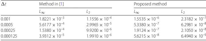
The maximum and Euclidean error norms corresponding to four diﬀerent values oft are reported in Table1usingN= 100 andα= 1.75. It is clear that the presented scheme approximates the exact analytical solution more precisely as compared to the method used

Table 1 Error norms for Problem1att= 1 withN= 100,α= 1.75

t Method in [1] Proposed method

L_∞ L2 L∞ L2

0.001 1.8221×10–3 1.1556×10–4 1.5535×10–6 2.3182×10–7

0.0005 5.6177×10–4 2.9965×10–5 5.3380×10–7 6.2981×10–8

0.00025 1.5380×10–4 9.9200×10–6 1.9124×10–7 2.1050×10–8

0.000125 3.9312_×10–5 _1.9910_×₁₀–6 _5.6215_×₁₀–8 _6.4940_×₁₀–9

Table 2 Error norms for Problem1, withN= 80 andt= 0.001

α t= 0.25 t= 0.5 t= 1

1.25 L2 2.5869×10–7 2.0680×10–7 1.5465×10–7

L_∞ 2.0113×10–6 _1.4491_×₁₀–6 _9.9176_×₁₀–7

1.50 L2 2.4923×10–7 2.2555×10–7 1.9223×10–7

L_∞ 2.0700×10–6 _1.6562_×₁₀–6 _1.2714_×₁₀–6

1.75 L2 2.3392×10–7 2.3887×10–7 2.3182×10–7

(16)

Table 3 Experimental order of convergence for Problem1, whenα= 1.50,N= 80,t= 0.001

N L∞ EOC L2 EOC

10 9.8950×10–2 _– _2.5950_×₁₀–2 _–

20 6.0451×10–3 4.0329 1.4778×10–3 4.1342

40 3.7842×10–4 3.9977 8.5142×10–5 4.1174

80 2.1927×10–5 4.1092 6.0168×10–6 3.8228

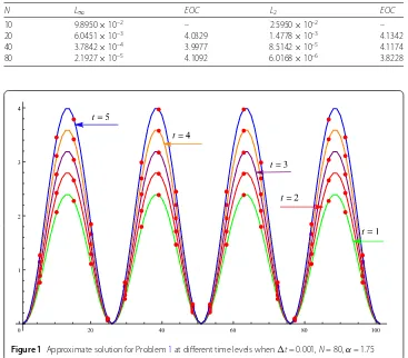
Figure 1Approximate solution for Problem1at diﬀerent time levels whent= 0.001,N= 80,α= 1.75

Figure 2Exact and numerical solution for Problem1withN= 80,t= 0.001, andα= 1.50

in [1]. In Table2, the error normsL∞andL2are listed att= 0.25, 0.5, 1 using diﬀerent

(17)

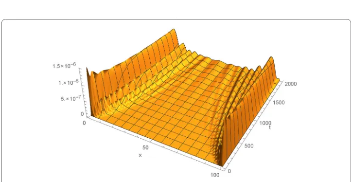
Figure 3Absolute error for Problem1whenN= 100,α= 1.75, andt= 0.0005

Figure 4Absolute error for Problem1whenN= 100,α= 1.5 andt= 1

with the exact solution, which indicates that the proposed method is eﬀective. Figure3 displays the absolute error att= 1 withα= 1.75 andN= 100, whereas Fig.4represents 3D error plot usingN= 100,α= 1.5, andt= 0.001.

Problem 2 As a second experiment, consider the following fourth order superdiﬀusion equation [1]:

∂α_y

∂tα +γ

∂4y

∂z4 =f(z,t), z∈[0, 1],t∈[0,T],

the initial/end conditions are

y(z, 0) = 1

π5

π10sin(πz) +cos(πz) –cos(3πz), y(0,t) =y(1,t) = 0,

yzz(0,t) =

1

π38(1 +t), yzz(1,t) = –

1

(18)

Table 4 Error norms for Problem2att= 1 withN= 80,α= 1.50

t Method in [1] Proposed method

L_∞ L2 L∞ L2

0.001 1.8221×10–3 _1.1556_×₁₀–4 _7.4454_×₁₀–8 _5.2661_×₁₀–8

0.0005 5.6177×10–4 _2.9965_×₁₀–5 _2.1479_×₁₀–8 _1.6911_×₁₀–8

0.00025 1.5380×10–4 _9.9200_×₁₀–6 _5.4476_×₁₀–9 _5.1349_×₁₀–9

0.000125 3.9312×10–5 _1.9910_×₁₀–6 _1.9831_×₁₀–9 _1.4734_×₁₀–9

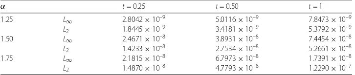
Table 5 Error norms for Problem2, whenN= 80 andt= 0.001

α t= 0.25 t= 0.50 t= 1

1.25 L_∞ 2.8042×10–9 _5.0116_×₁₀–9 _7.8473_×₁₀–9

L2 1.8445×10–9 3.4181×10–9 5.3792×10–9

1.50 L_∞ 2.4671×10–8 _3.8931_×₁₀–8 _7.4454_×₁₀–8

L2 1.4233×10–8 2.7534×10–8 5.2661×10–8

1.75 L_∞ 2.1815×10–8 _6.7973_×₁₀–8 _1.7391_×₁₀–8

L2 1.4870×10–8 4.7793×10–8 1.2290×10–7

Table 6 Experimental order of convergence for Problem2, whenN= 80,α= 1.50,t= 0.001

N L_∞ EOC L2 EOC

10 4.2119×10–4 _– _1.6769_×₁₀–4 _–

20 2.2034×10–5 _4.2566 _9.9991_×₁₀–6 _4.0678

40 1.8694×10–6 _4.1846 _6.9693_×₁₀–7 _3.8452

80 7.4454×10–8 _4.0245 _5.2661_×₁₀–8 _3.8605

The exact analytical solution to this problem is

y(z,t) = 1

π5

π10sin(πz) +cos(πz) –cos(3πz)(t+ 1).

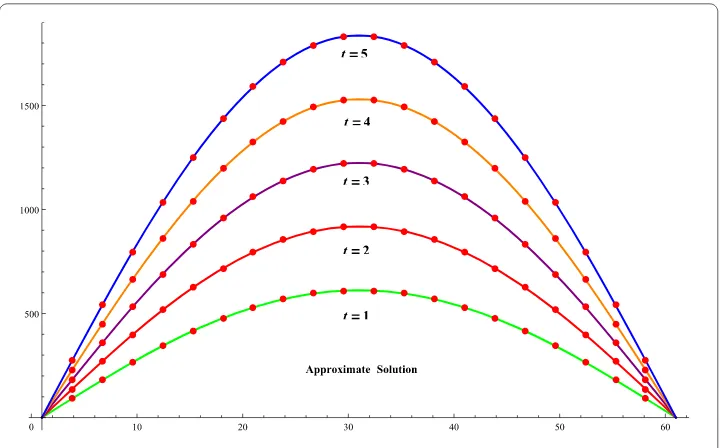
The computational error norms corresponding to four diﬀerent selections of t are given in Table4withγ = 0.05 andN= 80. It can be seen that our presented computa-tional strategy yields more accurate solutions as compared to the technique used in [1]. Table5shows the maximum and Euclidian error norms at diﬀerent time levels. The ex-perimental rate of convergence is tabulated in Table6when error norms are calculated forN= 80,α= 1.50, andt= 0.001. It is clear that the experimental results support the theoretical estimation. Figure5displays the approximate solution att= 1, 2, 3, 4, 5. The three-dimensional plots of analytical exact and numerical solutions are portrayed in Fig.6 in order to showcase their physical behaviour. In Fig.7, the absolute computational error is presented att= 1 usingα= 1.50 andN= 80.

7 Conclusion

1. An algorithm utilizing quintic non-polynomial spline functions has been developed for the numerical treatment of time fractional fourth order superdiﬀusion equation. 2. The discretization in space and time directions has been achieved by using quintic

non-polynomial spline functions and ﬁnite central diﬀerence formulation respectively.

3. The unconditional stability of the proposed scheme in temporal direction has been proved.

(19)

Figure 5Approximate solution for Problem2at diﬀerent time levels whent= 0.001,N= 60,α= 1.25

Figure 6Exact and numerical solution for Problem2whenN= 80,α= 1.25,t= 0.001

Figure 7Absolute error for Problem2whenN= 80,

t= 0.001 andα= 1.25

5. The experimental order of convergence is found to conform with the theoretical expectations.

(20)

Acknowledgements

The authors are also indebted to the anonymous reviewers for their helpful, valuable comments and suggestions in the improvement of this manuscript. This research was ﬁnancial supported by Research University grant

(1001/PMATHS/8011013) from School of Mathematical Sciences, Universiti Sains Malaysia.

Funding

All the ﬁnancial support for publishing this paper is funded by Universiti Sains Malaysia.

Availability of data and materials

Not applicable.

Competing interests

The authors declare that they have no competing interests.

Authors’ contributions

All authors equally contributed to this work. All authors read and approved the ﬁnal manuscript.

Authors’ information

Muhammad Amin is PhD scholar, Muhammad Abbas is Associate Professor, Muhammad Kashif Iqbal is Assistant Professor, Ahmad Izani Md. Ismail and Dumitru Baleanu are Professors.

Author details

1_{Department of Mathematics, National College of Business Administration & Economics, Lahore, Pakistan.}2_Department

of Mathematics, University of Sargodha, Sargodha, Pakistan. 3_{Department of Mathematics, Government College}

University, Faisalabad, Pakistan.4_{School of Mathematical Sciences, Universiti Sains Malaysia, Penang, Malaysia.} 5_{Department of Mathematics, Faculty of Arts and Sciences, Cankaya University, Ankara, Turkey.}6_{Department of Medical}

Research, China Medical University Hospital, China Medical University, Taichung, Taiwan. 7_{Institute of Space Sciences,}

Magurele-Bucharest, Romania.

Publisher’s Note

Springer Nature remains neutral with regard to jurisdictional claims in published maps and institutional aﬃliations.

Received: 19 September 2019 Accepted: 2 December 2019 References

1. Arshed, S.: Quintic b-spline method for time-fractional superdiﬀusion fourth-order diﬀerential equation. Math. Sci.

11(1), 17–26 (2017)

2. Tariq, H., Akram, G.: Quintic spline technique for time fractional fourth-order partial diﬀerential equation. Numer. Methods Partial Diﬀer. Equ.33(2), 445–466 (2017)

3. Podlubny, I.: Fractional Diﬀerential Equations: An Introduction to Fractional Derivatives, Fractional Diﬀerential Equations, to Methods of Their Solution and Some of Their Applications. Mathematics in Science and Engineering, vol. 198. Academic Press, San Diego (1998)

4. Miller, K.S., Ross, B.: An Introduction to the Fractional Calculus and Fractional Diﬀerential Equations. Wiley, New York (1993)

5. Jafari, H., Golbabai, A., Seiﬁ, S., Sayevand, K.: Homotopy analysis method for solving multi-term linear and nonlinear diﬀusion–wave equations of fractional order. Comput. Math. Appl.59(3), 1337–1344 (2010)

6. Dhaigude, D., Birajdar, G.A.: Numerical solution of system of fractional partial diﬀerential equations by discrete Adomian decomposition method. J. Fract. Calc. Appl.3(12), 1–11 (2012)

7. El-Sayed, A., Gaber, M.: The Adomian decomposition method for solving partial diﬀerential equations of fractal order in ﬁnite domains. Phys. Lett. A359(3), 175–182 (2006)

8. Momani, S., Odibat, Z.: Homotopy perturbation method for nonlinear partial diﬀerential equations of fractional order. Phys. Lett. A365(5–6), 345–350 (2007)

9. Turut, V., Güzel, N.: On solving partial diﬀerential equations of fractional order by using the variational iteration method and multivariate Padé approximations. Eur. J. Pure Appl. Math.6(2), 147–171 (2013)

10. Secer, A., Akinlar, M.A., Cevikel, A.: Efficient solutions of systems of fractional PDEs by the differential transform method. Adv. Differ. Equ.2012(1), 188 (2012)

11. Zahra, W.K., Elkholy, S.M.: The use of cubic splines in the numerical solution of fractional diﬀerential equations. Int. J. Math. Math. Sci.2012, Article ID 638026 (2012)

12. El Danaf, T.S.: Numerical solution for the linear time and space fractional diﬀusion equation. J. Vib. Control21(9), 1769–1777 (2015)

13. Siddiqi, S.S., Arshed, S.: Numerical solution of time-fractional fourth-order partial diﬀerential equations. Int. J. Comput. Math.92(7), 1496–1518 (2015)

14. Hamasalh, F.K., Muhammad, P.O.: Generalized quartic fractional spline interpolation with applications. Int. J. Open Problems Compt. Math.8(1), 67–80 (2015)

15. Mohyud-Din, S.T., Akram, T., Abbas, M., Ismail, A.I., Ali, N.H.: A fully implicit finite difference scheme based on extended cubic b-splines for time fractional advection–diffusion equation. Adv. Differ. Equ.2018(1), 109 (2018)

16. Li, M., Ding, X., Xu, Q.: Non-polynomial spline method for the time-fractional nonlinear Schrödinger equation. Adv. Diﬀer. Equ.2018(1), 318 (2018)

(21)

18. Khalid, N., Abbas, M., Iqbal, M.K.: Non-polynomial quintic spline for solving fourth-order fractional boundary value problems involving product terms. Appl. Math. Comput.349, 393–407 (2019)

19. Amin, M., Abbas, M., Iqbal, M.K., Baleanu, D.: Non-polynomial quintic spline for numerical solution of fourth-order time fractional partial diﬀerential equations. Adv. Diﬀer. Equ.2019(1), 183 (2019)

20. Khalid, N., Abbas, M., Iqbal, M.K., Baleanu, D.: A numerical algorithm based on modified extended B-spline functions for solving time-fractional diffusion wave equation involving reaction and damping terms. Adv. Differ. Equ.2019, 378 (2019)

21. Lin, Y., Xu, C.: Finite diﬀerence/spectral approximations for the time-fractional diﬀusion equation. J. Comput. Phys.

225(2), 1533–1552 (2007)

22. Iqbal, M.K., Abbas, M., Wasim, I.: New cubic b-spline approximation for solving third order Emden–Flower type equations. Appl. Math. Comput.331, 319–333 (2018)