R E S E A R C H A R T I C L E
Open Access
Numerical solution of fractional partial
differential equations by numerical Laplace
inversion technique
Mohammad Javidi
1and Bashir Ahmad
2**Correspondence:
[email protected] 2Department of Mathematics,
Faculty of Science, King Abdulaziz University, P.O. Box 80203, Jeddah, 21589, Saudi Arabia
Full list of author information is available at the end of the article
Abstract
In this paper, we propose a numerical method for solving fractional partial differential equations. This method is based on the homotopy perturbation method and Laplace transform. The transformed problem obtained by means of temporal Laplace transform is solved by the homotopy perturbation method. Then we use Stehfest’s numerical algorithm for calculating inverse Laplace transform to retrieve the time domain solution. The approximate solutions obtained by our proposed method are in excellent agreement with the exact solutions. It is worthwhile to note that our method is applicable to a variety of fractional partial differential equations occurring in fluid mechanics, signal processing, system identification, control robotics,etc.The utility of the method is shown by solving some interesting examples.
MSC: 34A08; 44A10
Keywords: Laplace transform; homotopy perturbation method; fractional PDEs; Stehfest’s algorithm
1 Introduction
Fractional differential equations are found to be an effective tool to describe certain phys-ical phenomena such as damping laws, rheology, diffusion processes, and so on. Several methods have been developed to solve fractional differential equations. Lin and Xu [] pro-posed the numerical solution for a time-fractional diffusion equation. In [], an uncondi-tionally stable finite element (FEM) approach for solving a one-dimensional Caputo-type fractional differential equation with singularity at the boundary was presented. Kexue and Jigen [] discussed the Laplace transform (LT) method for solving fractional differential equations with constant coefficients. Jafariet al.[] applied the homotopy analysis method to obtain the solution of a multi-order fractional differential equation in the Caputo sense. Merrikh-Bayat [] developed a low-cost numerical algorithm to find the series solution of nonlinear fractional differential equations with delay. In [], the Riemann-Liouville frac-tional integral for repeated fracfrac-tional integration was expanded in block pulse functions to yield the block pulse operational matrices for the fractional order integration. Esmaeiliet al.[] developed a computational technique based on the collocation method and Muntz polynomials for the solution of fractional differential equations. In [], three different nu-merical methods were used to solve a singularly perturbed Able Volterra integral equa-tion, presented by a fractional differential equation. Ibrahim [] discussed holomorphic solutions for nonlinear singular fractional differential equations.
Homotopy perturbation method (HPM) has been applied by several researchers to solve different kinds of functional equations. This method was further developed and improved by He [] and applied to develop a coupling method for a homotopy technique [], limit cycle and bifurcation of nonlinear problems [], nonlinear wave equation [], boundary value problems [], chemical kinetics system [], oscillators with discontinuities [], Riccati equation with fractional orders [], neutron transport equation [], nonlinear singular fourth order four-point boundary value problems [], systems of partial differ-ential equations [], nonlinear ill-posed operator equations [] and stiff systems of or-dinary differential equations [].
The Laplace transform method has been applied to a wide class of ordinary differen-tial equations (ODEs), pardifferen-tial differendifferen-tial equations (PDEs), integral equations (IEs) and integro-differential equations (IDEs). In these problems it is necessary to calculate the Laplace transform and inverse Laplace transform of certain functions. The inverse of Laplace transform is usually difficult to compute by using the techniques of complex anal-ysis, and there exist numerous numerical methods for its evaluation [, ]. Sastreet al.[] developed an application of Laguerre matrix polynomial series to the numerical inversion of Laplace transforms of matrix functions. Laguerre matrix polynomials were introduced in [] and theorems for the expansion of matrix functions in series of La-guerre matrix polynomials can be found in [, ]. In [], the dynamical differential equations with initial conditions were converted into the model of linear operator action, in which the linear operator is just the infinitesimal generator for the solver of the differen-tial equations, and the resolvent of the linear operator is the Laplace transform of the solver of original differential equations. In [], a method for the numerical inversion of Laplace transform on the real line of heavytailed (probability) density functions is presented. The method assumes a finite set of real values of the Laplace transform and chooses the an-alytical form of the approximant maximizing Shannon-entropy, so that positivity of the approximant itself is guaranteed. In [], a Laplace homotopy perturbation method is em-ployed for solving one-dimensional non-homogeneous partial differential equations with a variable coefficient. This method is a combination of the Laplace transform and the ho-motopy perturbation method (LHPM). LHPM presents an accurate methodology to solve non-homogeneous partial differential equations with a variable coefficient. Shenget al.
[] proposed an application of numerical inverse Laplace transform algorithms and ob-tained an easy way to solve the complicated fractional-order differential equations numer-ically.Weeksnumerical inversion of Laplace transform algorithm was established by using the Laguerre expansion and bilinear transformations []. The authors of [] developed an accurate numerical inversion of Laplace transforms. Tagliani [] proposed a numeri-cal method for inversion of Laplace transform with probability densities. The maximum entropy technique provides an analytical form of the approximate solution. Fractional mo-ments are mainly investigated. Entropy and cross-entropy convergence are proved. Valko
based on Laguerre polynomial series expansion of the inverse function under the assump-tion that the Laplace transform is known on the real axis only. The main contribuassump-tion of the paper is to provide computable estimates of truncation, discretization, conditioning and roundoff errors introduced by numerical computations. In the present work, we apply the Stehfest [] algorithm for numerical inversion of Laplace transform.
In this paper, the method for numerical solution of fractional partial differential equa-tions is based on Laplace transform (LT), the homotopy perturbation method (HPM) and Stehfest’s numerical algorithm for calculating inverse Laplace transform. The accuracy and efficiency of the method is verified by solving some examples of physical interest.
2 Homotopy perturbation technique
In this section, we describe the homotopy perturbation method [–] for a general type of the nonlinear differential equation with boundary conditions
A(u) –f(r) = , r∈, ()
B
u,∂u
∂n
= , r∈, ()
whereAis a general differential operator,Bis a boundary operator,f(r) is a known analyt-ical function andis the boundary of the domain. The operatorAcan be divided into two partsLandN, whereLis a linear operator andNis a nonlinear operator. Therefore, Eq. () can be rewritten as follows:
L(u) +N(u) –f(r) = . ()
By the homotopy technique, we define a homotopyH(r,p) :×[, ]→Ras follows:
H(u,p) = ( –p)L(u) –L(u)
+pA(u) –f(r)= , p∈[, ],r∈, () or
H(u,p) =L(u) –L(u) +pL(u) +p
N(u) –f(r)= , p∈[, ],r∈, () wherep∈[, ] is an embedding parameter, anduis an initial approximation for Eq. () with
H(u, ) =L(u) –L(u) = , H(u, ) =A(u) –f(r) = . ()
Note that the process of varying the values ofpfrom zero to unity corresponds to that of
u(r,p) fromu(r) tou(r). We assume that the solution of Eq. () can be written as a power series inp, that is,
v=
∞
k=
pkuk. ()
3 Preliminaries
In this section, we recall some basic concepts of fractional calculus [–] and Laplace transform.
Definition Forμ∈R, a functionf :R→R+is said to be in the spaceC
μif it can be
written asf(x) =xpf
(x) withp>μ,f(x)∈C[,∞), and it is said to be in the spaceCmμ if
f(m)∈Cμform∈N∪ {}.
Definition The Riemann-Liouville fractional integral of orderα> for a functionf ∈ Cμwithμ≥– is defined as
Jαf(t) =
(α)
t
(t–τ)α–f(τ)dτ, α> ,t> ,
Jf(t) =f(t).
()
Definition The Riemann-Liouville fractional derivative of orderα> for a function
f ∈C–m withm∈N∪ {}is defined as
Dα∗f(t) = d m
dtmJ m–α
f(t), m– <α≤m,m∈N. ()
Definition The Caputo fractional derivative of orderα> for a functionf ∈Cm –with
m∈N∪ {}is defined as
Dαf(t) =
⎧ ⎨ ⎩
Jm–αf(m)(t), m– <α≤m,m∈N, dmf(t)
dtm , α=m.
()
Definition A two-parameter Mittag-Leffler function is defined by the following series:
Eα,β(t) =
∞
k=
tk
(αk+β). ()
Observe thatE,(t) =et,E,(–t) =e–t.
Definition The Laplace transform of a functionu(x,t),t≥, denoted byϕ(x,s), is de-fined by
Lu(x,t)=ϕ(x,s) =
∞
e–stu(x,t)dt, ()
wheresis the transform parameter and is assumed to be real and positive. Note that the Laplace transform of Mittag-Leffler functionEα,β(t) is
LEα,β(t)
=
∞
e–stEα,β(t)dt=
∞
k=
(k+ )
The Laplace transform ofDαf(t) can be found as follows:
4 Description of the method
Consider the following linear fractional partial differential equation:
∂αu andm– <α≤m. Now we explain the method of solution for solving initial-boundary value problem ()-().
Taking the Laplace transform of problem ()-() and using (), we obtain
Rewriting Eq. (), we have
According to HPM, we construct a homotopy for Eq. () as follows:
Then the solution of Eq. () can be expressed as
(x,s) =
which, on comparing the coefficients of powers ofp, yields
p: (x,s) =
In the limitp→, we note that () becomes the approximate solution for the problem of ()-() and is given by
Taking the inverse Laplace transform of (), we obtain
Applying Stehfest’s algorithm [] toHn(x,s), the solutionu(x,t) is found to be
wherepis a positive integer and
dj= (–)j+p min(j,p) i=[j+ ]
ip(i)!
(p–i)!i!(i– )!(j–i)!(i–j)!.
Here [r] denotes the integer part of the real numberr.
5 Numerical results
In this section, we show the efficiency and accuracy of the new Laplace homotopy pertur-bation method (LHPM) by applying it to several test problems.
Example Consider the following initial-boundary value problem [].
∂αu
We know that the exact solution of this problem is
u(x,t) =x+x
By using the method developed in the previous section (), we find that
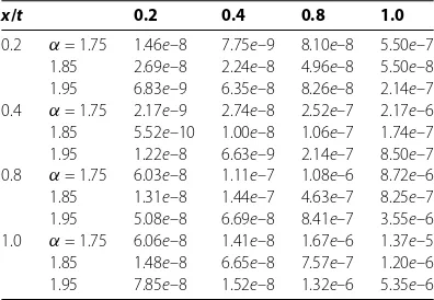
Table 1 Absolute errors|u(x,t) –un(x,t)|by LHPM withp= 8,α= 1.75, 1.85, 1.95,n= 3 for various values ofxandtfor Example 1
x/t 0.2 0.4 0.8 1.0
0.2 α= 1.75 1.46e–8 7.75e–9 8.10e–8 5.50e–7 1.85 2.69e–8 2.24e–8 4.96e–8 5.50e–8 1.95 6.83e–9 6.35e–8 8.26e–8 2.14e–7 0.4 α= 1.75 2.17e–9 2.74e–8 2.52e–7 2.17e–6 1.85 5.52e–10 1.00e–8 1.06e–7 1.74e–7 1.95 1.22e–8 6.63e–9 2.14e–7 8.50e–7 0.8 α= 1.75 6.03e–8 1.11e–7 1.08e–6 8.72e–6 1.85 1.31e–8 1.44e–7 4.63e–7 8.25e–7 1.95 5.08e–8 6.69e–8 8.41e–7 3.55e–6 1.0 α= 1.75 6.06e–8 1.41e–8 1.67e–6 1.37e–5 1.85 1.48e–8 6.65e–8 7.57e–7 1.20e–6 1.95 7.85e–8 1.52e–8 1.32e–6 5.35e–6
Taking the inverse Laplace transform of (), the approximate solution of ()-() is given by
un(x,t) =L–Hn(x,s)=x+x
n
k=
tkα+
(kα+ ), ()
which, on taking the limitn→ ∞, yields
u(x,t) = lim
n→∞un(x,t) =x+x
∞
k=
tkα+
(kα+ ). ()
Table shows the absolute errors|u(x,t) –un(x,t)|using the LHPM with p= ,α= ., ., .,n= for various values ofxandt. Clearly, it follows from the table that the numerical solutions are in good agreement with the exact solution.
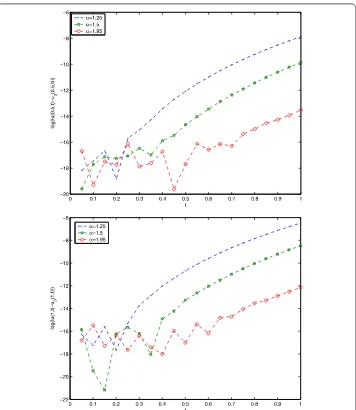
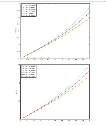
In Figure , we plot the logarithm of absolute errors obtained by the LHPM atx= ., withn= ,p= for various values oft. In Figure , we plot the numerical solution and the exact solution atx= ., withn= ,p= for various values ofαandt.
Example Let us consider the following fractional differential equation [].
∂αu
∂tα +x
∂u ∂x+
∂u ∂x =
tα+x+ , <t≤, ≤x≤, <α≤, () with the initial condition
u(x, ) =x ()
and the boundary conditions
u(,t) = tα (α+ )
(α+ ), u(,t) = + t
α (α+ )
(α+ ). ()
The exact solution of the given problem is given by
u(x,t) =x+ tα (α+ )
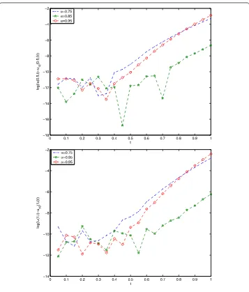
Figure 1 Logarithm of absolute errors obtained by the LHPM atx= 0.5, 1 withn= 10,p= 8 for various values oft.
By using the method presented in Section , namely (), we obtain
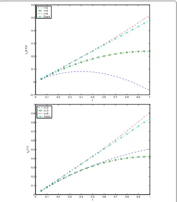
Figure 2 The numerical solution and the exact solution atx= 0.5, 1 withn= 3,p= 8 for various values ofαandt.
As before, by using (), we obtain
Hn(x,s) =
(α+ )
sα+ +
x
s + (–)
n +x n+
s(n+)α+. ()
Taking the inverse Laplace transform of () and taking the limitn→ ∞, the approximate solution for problem ()-() is given by
u(x,t) = lim
n→∞un(x,t) =x
+ tα (α+ )
(α+ ). ()
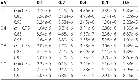
In Table , we list the absolute errors using the LHPM withp= ,α= ., ., .,
Table 2 Absolute errors by LHPM withp= 10,α= 0.75, 0.85, 0.95,n= 10 for various values of
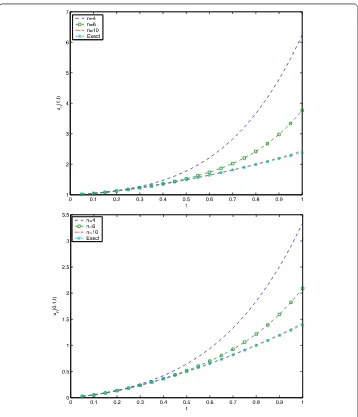
In Figure , we plot the logarithm of absolute errors obtained by the LHPM atx= ., withn= ,p= for various values oft. In Figure , we plot the exact solution and the numerical solution obtained by the LHPM withx= ., forn= , , ,p= ,α= . for various values oft. As we see from Figure , the numerical solutions are in good agreement with the exact solution as the value ofnis increased.
Example Consider the fractional differential equation []
∂αu
The exact solution for this problem is
u(x,t) =tsin(x). ()
Following the method of Section (), we find that
Figure 3 Logarithm of absolute errors obtained by the LHPM atx= 0.5, 1 withn= 10,p= 10 for various values oft.
By means of (), we obtain
Hn(x,s) =(α+ )
sα+ +
x s + (–)
n +x n+
s(n+)α+. ()
Taking the inverse Laplace transform of (), the approximate solution of ()-() is found to be
un(x,t) =L–
Hn(x,s)
=
⎧ ⎨ ⎩
sinx
s +s(ncosx+)α+, n= k, sinx(s –s(n+)α+), n= k+ ,
()
which, on taking the limitn→ ∞, gives
u(x,t) = lim
Figure 4 The exact solution and the numerical solution obtained by the LHPM withx= 0.1, 1 for
n= 4, 6, 10,p= 10,α= 0.75 for various values oft.
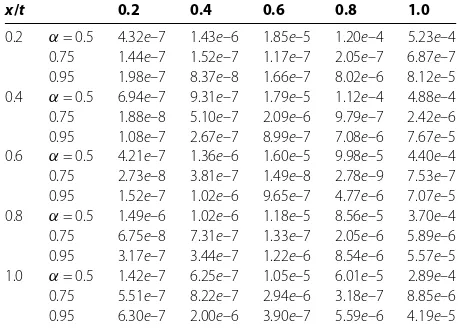
In Table , we list the absolute errors using the LHPM withp= ,α= ., ., .,
n= for various values ofxandt. It follows from the table that the numerical solutions are in good agreement with the exact solution.
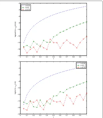
In Figure , we plot the logarithm of absolute errors obtained by the LHPM atx= ., withn= ,p= for various values oft. In Figure , we plot the exact solution and the numerical solution obtained by the LHPM withx= ., forn= , , ,p= ,α= . for various values oft. Clearly, the numerical solutions are in good agreement with the exact solution as the value ofnis increased.
Example Consider the fractional differential equation
∂αu
∂tα(x,t) +u
(x,t) = xt–α
( –α)+x
Table 3 Absolute errors by LHPM withp= 10,α= 0.5, 0.75, 0.95,n= 10 for various values ofx
andtfor Example 3
x/t 0.2 0.4 0.6 0.8 1.0
The exact solution for this problem is
u(x,t) =xt. ()
Taking the Laplace transform of problem ()-() and using (), we obtain
According to HPM, we construct a homotopy for Eq. () as follows:
(x,s) =
Following the method of Section (), we find that
Figure 5 Logarithm of absolute errors obtained by the LHPM atx= 0.5, 1 withn= 10,p= 10 for various values oft.
(x,s) =
×!x
sα+(α+ )
(α+ ) + !(α+ )(α+ )
(α+ )(α+ )sα+
+ x(α+ )(α+ )
(α+ )sα+
+ ! x(α+ )
(α+ )sα+ + (!)
x(α+ )(α+ )
(α+ )(α+ )sα+
and so on.
By means of (), we obtain
H(x,s) = x
s +
×!x
sα+(α+ )
!(α+ )(α+ )
(α+ )(α+ )sα+
+ x(α+ )(α+ )
(α+ )sα+ + (!)
x(α+ )(α+ )
(α+ )(α+ )sα+
Figure 6 The exact solution and the numerical solution obtained by the LHPM withx= 0.5, 1 for
n= 2, 3, 9,p= 10,α= 0.25 for various values oft.
Taking the inverse Laplace transform of (), the approximate solution of ()-() is found to be
un(x,t) =L–
Hn(x,s)
=xt+ ×!x
(α+ )(α+ )
(α+ )(α+ )(α+ )t α+
+ ×! x
(α+ )(α+ )
(α+ )(α+ )(α+ )t α+
+ (!) x
(α+ )(α+ )
(α+ )(α+ )(α+ )t
α+. ()
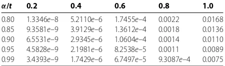
In Table , we list the absolute errors using the LHPM withα= ., ., ., ., .,
Table 4 Absolute errors by LHPM withα= 0.8, 0.85, 0.90, 0.95, 0.99,n= 2,x= 0.5 for various values oftfor Example 4
α/t 0.2 0.4 0.6 0.8 1.0
0.80 1.3346e–8 5.2110e–6 1.7455e–4 0.0022 0.0168 0.85 9.3581e–9 3.9129e–6 1.3612e–4 0.0018 0.0136 0.90 6.5531e–9 2.9345e–6 1.0604e–4 0.0014 0.0110 0.95 4.5828e–9 2.1981e–6 8.2538e–5 0.0011 0.0089 0.99 3.4393e–9 1.7429e–6 6.7497e–5 9.3087e–4 0.0075
6 Conclusions
In this paper, we have developed a new numerical method for solving fractional partial differential equations. This method is based on Laplace transform, the homotopy pertur-bation method and Stehfest’s numerical algorithm for calculating inverse Laplace trans-form. We demonstrate the efficiency and accuracy of the proposed method by applying it to three typical examples. It is found that the approximate solutions produced by our method are in complete agreement with the corresponding exact solutions. Moreover, in view of its simplicity, our method is applicable to a wide class of initial-boundary value problems occurring in applied sciences.
Competing interests
The authors declare that they have no competing interests.
Authors’ contributions
Each of the authors, MJ and BA contributed to each part of this work equally and read and approved the final version of the manuscript.
Author details
1Faculty of Mathematical Sciences, University of Tabriz, Tabriz, Iran.2Department of Mathematics, Faculty of Science, King
Abdulaziz University, P.O. Box 80203, Jeddah, 21589, Saudi Arabia.
Acknowledgements
The authors thank the reviewers for their constructive remarks that led to the improvement of the original manuscript. The research of Bashir Ahmad was partially supported by the Deanship of Scientific Research (DSR), King Abdulaziz University, Jeddah, Saudi Arabia.
Received: 4 October 2013 Accepted: 25 November 2013 Published:20 Dec 2013
References
1. Lin, Y, Xu, C: Finite difference/spectral approximations for the time-fractional diffusion equation. J. Comput. Phys.225, 1533-1552 (2007)
2. Huang, Q, Huang, G, Zhan, H: A finite element solution for the fractional advection-dispersion equation. Adv. Water Resour.31, 1578-1589 (2008)
3. Kexue, L, Jigen, P: Laplace transform and fractional differential equations. Appl. Math. Lett.24, 2019-2023 (2011) 4. Jafari, H, Das, S, Tajadodi, H: Solving a multi-order fractional differential equation using homotopy analysis method.
J. King Saud Univ., Sci.23, 151-155 (2011)
5. Merrikh-Bayat, F: Low-cost numerical algorithm to find the series solution of nonlinear fractional differential equations with delay. Proc. Comput. Sci.3, 227-231 (2011)
6. Li, Y, Sun, N: Numerical solution of fractional differential equations using the generalized block pulse operational matrix. Comput. Math. Appl.62(3), 1046-1054 (2011)
7. Esmaeili, S, Shamsi, M, Luchko, Y: Numerical solution of fractional differential equations with a collocation method based on Müntz polynomials. Comput. Math. Appl.62(3), 918-929 (2011)
8. Erjaee, GH, Taghvafard, H, Alnasr, M: Numerical solution of the high thermal loss problem presented by a fractional differential equation. Commun. Nonlinear Sci. Numer. Simul.16, 1356-1362 (2011)
9. Ibrahim, RW: On holomorphic solutions for nonlinear singular fractional differential equations. Comput. Math. Appl.
62(3), 1084-1090 (2011)
10. He, JH: Homotopy perturbation technique. Comput. Methods Appl. Mech. Eng.178, 257-262 (1999)
11. He, JH: A coupling method of a homotopy technique and a perturbation technique for non-linear problems. Int. J. Non-Linear Mech.35(1), 37-43 (2000)
12. He, JH: Limit cycle and bifurcation of nonlinear problems. Chaos Solitons Fractals26(3), 827-833 (2005)
13. He, JH: Application of homotopy perturbation method to nonlinear wave equations. Chaos Solitons Fractals26(3), 695-700 (2005)
15. Aminikhah, H: An analytical approximation to the solution of chemical kinetics system. Journal of King Saud University Science23, 167-170 (2011)
16. He, JH: The homotopy perturbation method for non-linear oscillators with discontinuities. Appl. Math. Comput.
151(1), 287-292 (2004)
17. Khan, NA, Ara, A, Jamil, M: An efficient approach for solving the Riccati equation with fractional orders. Comput. Math. Appl.61, 2683-2689 (2011)
18. Martin, O: A homotopy perturbation method for solving a neutron transport equation. Appl. Math. Comput.217, 8567-8574 (2011)
19. Li, XY, Wu, BY: A novel method for nonlinear singular fourth order four-point boundary value problems. Comput. Math. Appl.62, 27-31 (2011)
20. Biazar, J, Eslami, M: A new homotopy perturbation method for solving systems of partial differential equations. Comput. Math. Appl.62, 225-234 (2011)
21. Cao, L, Han, B: Convergence analysis of the homotopy perturbation method for solving nonlinear ill-posed operator equations. Comput. Math. Appl.61, 2058-2061 (2011)
22. Aminikhah, H, Hemmatnezhad, M: An effective modification of the homotopy perturbation method for stiff systems of ordinary differential equations. Appl. Math. Lett.24, 1502-1508 (2011)
23. Cohen, AM: Numerical Methods for Laplace Transform Inversion. Springer, Berlin (2007)
24. Davies, B, Martin, B: Numerical inversion of Laplace transform: a survey and comparison of methods. J. Comput. Phys.
33, 1-32 (1979)
25. Sastre, J, Defez, E, Jodar, L: Application of Laguerre matrix polynomials to the numerical inversion of Laplace transforms of matrix functions. Appl. Math. Lett.24, 1527-1532 (2011)
26. Jódar, L, Company, R, Navarro, E: Laguerre matrix polynomials and systems of second order differential equations. Appl. Numer. Math.15, 53-63 (1994)
27. Sastre, J, Defez, E, Jódar, L: Laguerre matrix polynomials series expansion: theory and computer applications. Math. Comput. Model.44, 1025-1043 (2006)
28. Sastre, J, Jódar, L: On Laguerre matrix polynomials series. Util. Math.71, 109-130 (2006)
29. Suying, Z, Minzhen, Z, Zichen, D, Wencheng, L: Solution of nonlinear dynamic differential equations based on numerical Laplace transform inversion. Appl. Math. Comput.189, 79-86 (2007)
30. Tagliani, A, Velasquez, Y: Numerical inversion of the Laplace transform via fractional moments. Appl. Math. Comput.
143, 99-107 (2003)
31. Madani, M, Fathizadeh, M, Khan, Y, Yildirim, A: On the coupling of the homotopy perturbation method and Laplace transformation. Math. Comput. Model.53, 1937-1945 (2011)
32. Sheng, H, Li, Y, Chen, Y: Application of numerical inverse Laplace transform algorithms in fractional calculus. J. Franklin Inst.348, 315-330 (2011)
33. Weeks, WT: Numerical inversion of Laplace transforms using Laguerre functions. J. ACM13(3), 419-429 (1966) 34. Talbot, A: The accurate numerical inversion of Laplace transforms. J. Appl. Math.23(1), 97-120 (1979)
35. Tagliani, A: Numerical inversion of Laplace transform on the real line from expected values. Appl. Math. Comput.134, 459-472 (2003)
36. Valko, PP, Abate, J: Numerical Laplace inversion in rheological characterization. J. Non-Newton. Fluid Mech.116, 395-406 (2004)
37. Mahajerin, E, Burgess, G: A Laplace transform-based fundamental collocation method for two-dimensional transient heat flow. Appl. Therm. Eng.23, 101-111 (2003)
38. Cuomo, S, D’Amore, L, Murli, A, Rizzardi, M: Computation of the inverse Laplace transform based on a collocation method which uses only real values. J. Comput. Appl. Math.198, 98-115 (2007)
39. Stehfest, H: Algorithm 368: numerical inversion of Laplace transform. Commun. ACM13(1), 47-49 (1970) 40. Podlubny, I: Fractional Differential Equations. An Introduction to Fractional Derivatives, Fractional Differential
Equations, to Methods of Their Solution and Some of Their Applications. Academic Press, San Diego (1999) 41. Diethelm, K: The Analysis of Fractional Differential Equations. Springer, Berlin (2010)
42. Kilbas, AA, Srivastava, HM, Trujillo, JJ: Theory and Applications of Fractional Differential Equations. North-Holland Mathematics Studies, vol. 204. Elsevier, Amsterdam (2006)
43. Kiryakova, V: Generalized Fractional Calculus and Applications. Pitman Research Notes in Math., vol. 301. Longman, Harlow (1994)
44. Miller, KS, Ross, B: An Introduction to the Fractional Calculus and Fractional Differential Equations. Wiley, New York (1993)
45. Karimi-Vanani, S, Aminataei, A: Tau approximate solution of fractional partial differential equations. Comput. Math. Appl.62(3), 1075-1083 (2011)
46. Moaddy, K, Momani, S, Hashim, I: The non-standard finite difference scheme for linear fractional PDEs in fluid mechanics. Comput. Math. Appl.61, 1209-1216 (2011)
10.1186/1687-1847-2013-375