Numerical solution for a class of multi order fractional differential equations with error correction and convergence analysis

R E S E A R C H

Open Access

Numerical solution for a class of

multi-order fractional differential equations

with error correction and convergence

analysis

Wei Han

_{, Yi-Ming Chen}

_{, Da-Yan Liu}

_{, Xiao-Lin Li}

_{and Driss Boutat}

*_{Correspondence:}

[email protected]

1_{School of Sciences, Yanshan}

University, Qinhuangdao, P.R. China

2_{Loire Valley Institute for Advanced}

Studies, Orléans, France Full list of author information is available at the end of the article

Abstract

In this article, we investigate numerical solution of a class of multi-order fractional differential equations with error correction and convergence analysis. According to fractional differential definition in Caputo’s sense, fractional differential operator matrix is deduced. The problem is reduced to a set of algebraic equations, and we apply MATLAB to solve the equation. In order to improve the precision of numerical solution, the process of error correction for multi-order fractional differential equation is introduced. By constructing the multi-order fractional differential equation of the error function, the approximate error function is obtained so that the numerical solution is corrected. Then, we analyze the convergence of the shifted Chebyshev polynomials approximation function. Numerical experiments are given to demonstrate the applicability of the method and the validity of error correction.

Keywords: Shifted Chebyshev polynomials; Multi-order fractional differential equation; Error correction; Convergence analysis; Numerical solution

1 Introduction

Fractional calculus [1] is developing fast and its various applications are extensively used in many fields of science and engineering. It has been applied to chaotic systems [2,3] and optimal control problems [4]. In [5], the authors derived the fractional Euler–Lagrange equation in terms of the Caputo fractional derivatives. Kumar et al. [6] analyzed Fornberg– Whitham equation pertaining to a fractional derivative with Mittag–Leffler type kernel. The authors of [7] investigated a time-fractional modified Kawahara equation through a fractional derivative with exponential kernel. In [8] Singh et al. presented a fractional epi-demiological model and solved the solution of the problem by using an iterative method. Fractional differential equation [9] is used to describe mathematical phenomena of many areas, such as rheology, damping method, signal processing, control theory, poly-mers, viscoelastic materials, and so on. Many researchers [10,11] focus on the numer-ical treatments of fractional differential equation, such as homotopy analysis transform method [12,13], iterative reproducing kernel Hilbert space method [14], artificial neural network approach [15], variational iteration method and its modification [16], Wavelet

method [17–19], Bernstein polynomials [20], and fractional-order Legendre functions [21]. The authors of [22] researched space–time fractional Rosenou–Haynam equation. In [23] Baleanu et al. solved the time fractional third-order evolution (TOE) equation with Riemann–Liouville (RL) derivative.

Since multi-order fractional differential equations are applied in many fields, many sci-entists have begun to study the properties and numerical solutions of equations. Multi-order fractional differential equation [24] is one of the most important types of fractional differential equations. Authors of [25,26] investigated the existence, uniqueness, conver-gence of the solution for multi-order fractional differential equation. Because there is no exact solution, most different numerical methods, such as stable fractional Chebyshev differentiation matrix [27], fractional-order operational method [28], spectral collocation methods [29], and so on, have been used to investigate the approximate solutions of multi-order fractional differential equation. The authors of [30] only researched the convergence effect of numerical solutions and exact solutions of equations. There is little literature with shifted Chebyshev polynomials to solve multi-order fractional differential equation and research error correction and convergence. In this paper, the numerical solutions of a class of multi-order fractional differential equations with error correction and conver-gence analysis are investigated. According to the function approximation theory and frac-tional differential operator matrix, the equation is transformed into algebraic equations. The correction solutions of multi-order fractional differential equation are investigated and the convergence of the shifted Chebyshev polynomials approximation function is an-alyzed. We do the correction for the numerical solution of low precision and obtain the absolute error of the correction solution, so that the accuracy of the numerical solution is improved.

In general, multi-order fractional differential equation is expressed as follows:

Dαu(x) = k

i=0

yiDβiu(x) +f(x), x∈[0, 1]

with the initial conditions

u(p)(0) =dp, p= 0, 1, . . . ,n– 1,

wheren– 1 <α≤n, the coefficientyi(i= 0, 1, . . . ,k) is constant, and 0 <β0<· · ·<βk<α,

f(x) is a known function.

The rest of the paper is organized as follows: Sect.2introduces the definition of Caputo fractional derivatives and shifted Chebyshev polynomials. In Sect.3, the function approx-imation theory is introduced. In Sect.4, the process of error correction for multi-order fractional differential equation is introduced and the convergence of the shifted Cheby-shev polynomials approximation function is analyzed. Section5 deduces the fractional differential operator matrix based on shifted Chebyshev polynomials. Section6reduces the problem to a set of algebraic equations. In Sect.7, the proposed method is applied to two examples. Conclusion is given in Sect.8.

2 Preliminary knowledge

2.1 The Caputo fractional derivatives

Definition 1 The Caputo fractional derivative operatorDα

x of orderα is defined in the

For Caputo’s derivatives, we have

C aD

α

xC= 0, (2)

whereCis a constant.

C

2.2 Shifted Chebyshev polynomials

The well-known Chebyshev polynomials can be defined on the intervalx∈[–1, 1] and can be determined with the following recurrence formula:

⎧ ⎨ ⎩

P∗₀(x∗) = 1, P₁∗(x∗) =x∗

P∗_i+1(x∗) = 2x∗P_i∗(x∗) –P_i∗_–1(x∗), i= 1, 2, 3, . . . . (4)

In order to obtain these polynomials on the interval [0, 1], we introduce the change of variablex∗= 2x– 1 and substitutex∗toP_i∗(x∗),i= 0, 1, 2, . . . . The shifted Chebyshev poly-nomials can be defined as

⎧

The shifted Chebyshev polynomialsPn(x) of degree n can be given by

Pn(x) =

the weight function is

ws(x) = 1

√

x–x2. (7)

Combining (7) the orthogonality condition is

We can define the shifted Chebyshev vector as follows:

(x) =P0(x),P1(x), . . . ,Pn(x) T, (9)

the vector is represented as a matrix form as follows:

(x) =ATn(x), (10)

The functionu(x) is a continuous function which can be expanded in shifted Chebyshev polynomials:

A finite expansion in the first (n+ 1)-term shifted Chebyshev polynomials is

u(x)∼= n

i=0

ciPi(x) =CT(x), (11)

where the shifted Chebyshev vector(x) and the shifted Chebyshev coefficient vectorC

are given by

C= [c0,c1, . . . ,cn]T,

(x) =P0(x),P1(x), . . . ,Pn(x) T

.

The coefficient vectorCcan be determined by the inner product

C=Q–1u,(x),

where the inner product is defined as

f,(x)= xf

0

whereQis

4 Error correction and convergence analysis

In this section, we do error correction for multi-order fractional differential equation and introduce convergence of shifted Chebyshev polynomials. The order of convergence isn.

4.1 Error correction

We solve multi-order fractional differential equation via the shifted Chebyshev polyno-mials. If the absolute error between the numerical solution and exact solution is larger, according to the correct solution and the exact solution, we can get the absolute error of correct solution. Error correction improves the precision of numerical solution.

We assume that the numerical solution of multi-order fractional differential equation is

uM(x), the exact solution isu(x), the error between the numerical solution and the exact solution is

eM(x) =u(x) –uM(x), (12)

whereeM(x) is an error function.

Substituting the numerical solution of equationuM(x) in multi-order fractional differ-ential equation, we can get

DαuM(x)≈ k

i=0

yiDβiuM(x) +f(x). (13)

A residual functionwM(x) is added to the right-hand side of the multi-order fractional differential equation, (13) can be transformed into

DαuM(x) = k

i=0

Then we can get the equation

QuM(x) =f(x) +wM(x), (15)

where

QuM(x) =DαuM(x) – k

i=0

yiDβiuM(x). (16)

We assume thatφis the unknown variables in the following equation:

Q[φ] =Dαφ– k

i=0

yiDβiφ, (17)

whenφ=u(x) andφ=eM(x), we have

Qu(x) =Dαu(x) – k

i=0

yiDβiu(x) =f(x), (18)

QeM(x) =DαeM(x) – k

i=0

yiDβieM(x). (19)

Combining (12) and (15)–(19), we can obtain

QeM(x) =Q

u(x) –QuM(x) = –wM(x). (20)

According to (19) and (20), we can get

DαeM(x) – k

i=0

yiDβieM(x) = –wM(x). (21)

We name (21) multi-order fractional differential equation of error function.eM(x) is the exact solution,e∗ω(x) is the numerical solution, namely the approximate error function.

According to the numerical solution of multi-order fractional differential equation

uM(x) and the numerical solution of multi-order fractional differential equation of error functione∗ω(x), correct solutionu∗(x) can be obtained:

u∗(x) =uM(x) +e∗ω(x). (22)

Combining (22) with the exact solutionu(x), we can get the absolute error of correct solution:

er(x)=u(x) –u∗(x). (23)

The errorer(x) between the exact solution and the numerical solution of multi-order fractional differential equation of error function is

er(x) =eM(x) –e∗ω(x) =u(x) –uM(x) –e∗ω(x) (24)

In the same way, according to the shifted Chebyshev polynomials function approxima-tion theory, correct soluapproxima-tionu∗(x) can be translated into a matrix form as follows:

u∗(x)∼=

Definition 2 In the interval [a,b], we can define arbitrary function convergence coeffi-cient of form as follows:

ω(f,δ) = sup

Theorem 3 When f(x)satisfiesαorder Lipschitz condition in[0, 1],then there is

f –q(f,n)∞≤3 2km

–α2_,

where k is a Lipschitz constant.

Theorem 4 If f(x)is bounded on[0, 1],Y=Span{P0,P1,P2, . . . ,Pn}.If CT(x)is the best

approximation of f in the linear space Y,then there is

_{f –c}T

5 Fractional differential operator matrix

According to (10), the differential operator can be derived as follows:

D(x) =DATn(x)

The above formula can be shown specifically as follows:

Q(n+1)×n=

First-order differential operator matrix is

where

So the fractional differential operator can be deduced

Dβ2_{(x) =ANA}–1_{(x) =G(x). (28)}

Fractional differential operator matrix is

G=ANA–1. (29)

6 The numerical algorithm

The multi-order fractional differential equation, which we study in this paper, can be ex-pressed as follows:

Dαu(x) =y0Dβ0_{u(x) +y1D}β1_{u(x) +y2D}β2_u(x)

+y3Dβ3u(x) +f(x), x∈[0, 1] (30)

with the initial conditions

u(0)(0) =d0, u(1)(0) =d1, (31)

whereα= 2,k= 3, the coefficientyi(i= 0, 1, 2, 3) is constant, andβ0= 0,β1= 1, 0 <β2< 1, 1 <β3< 2,f(x) is a known function.

On the basis of (10), (11), (26), the item in equation can be converted into the matrix, we can deduce concretely them as follows:

Du(x)∼= DCT(x) =CTAQ(n+1)×nB∗(x) =CTE(x), (32)

D2u(x)∼= D2CT(x) =CTD2(x) =CTD2ATn(x)

=CTE2(x). (33)

Then, the second-order differential operator matrix is

Whenβ3∈(1, 2), (β2<β3), that is to sayβ2=β3– 1∈(0, 1), according to (10), (11), (26), (28), the item in equation can be converted into the matrix as follows:

Dβ3_u(x)∼_{= D}β3_CT_{(x) = D}β2_DCT_(x)=CT_Dβ2_E(x)

=CTEDβ2_{(x) =C}T_EANA–1_{(x) =C}T_{EG(x), (35)}

where

K=EANA–1=EG. (36)

Combining (11) with (32)–(36), the equation can be converted into

CTE2(x) =y0CT(x) +y1CTE(x) +y2CTG(x) +y3CTK(x) +f(x).

Also, we substitute the correction solution into the original equation and translate the original equation into matrix as follows:

C∗TE2∗(x) =y0

C∗T∗(x) +y1

C∗TE∗(x)

+y2

C∗TG∗(x) +y3

C∗TK∗(x) +f(x).

By using the collocation method, the variables are discretized, the problem can be trans-ferred to linear equations. Combining MATLAB software with least square method to solve the unknown coefficient, numerical solution of the problem can be obtained.

7 Numerical examples

In this section, two experiments prove that the proposed method is effective and feasible.

Example1 Consider the following multi-order fractional differential equation:

Dαu(x) =y0Dβ0_{u(x) +y1D}β1_{u(x) +y2D}β2_u(x)

+y3Dβ3_{u(x) +f(x), x}∈_{[0, 1],}

with the initial conditions

u(0)(0) =d0,u(1)(0) =d1,

whereα= 2,d0=d1= 0, the coefficient isy0=y2= –1,y1= 2,y3= 0, andβ0= 0,β1= 1,

β2=1₂∈(0, 1), the known function is

f(x) =x7+ 2048 429√πx

6.5_{– 14x}6_{+ 42x}5_–x2_– 8 3√πx

1.5_{+ 4x– 2,}

the exact solution isu(x) =x7_–x2_.

0.1750, 0.0924]T_{, the shifted Chebyshev polynomials of approximation function(x) are} 0.1220, 0.0441, 0.0113, 0.0020]T, the shifted Chebyshev polynomials of approximation function(x) are 0.1222, 0.0444, 0.0111, 0.0017, 0.0001]T_{, the shifted Chebyshev polynomials of} approxima-tion funcapproxima-tion(x) are

Compared with [30], Example1studies the approximation effect of numerical solution and exact solution, the absolute errors and the absolute error of correct solution. When

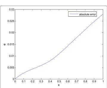
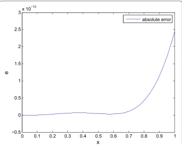
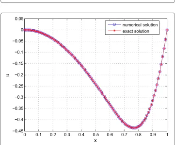
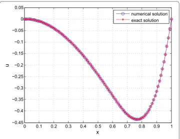
n= 4, 6, 7, the absolute errors for equation in some match points between the numerical solution and the exact solution are shown in Fig.1–Fig.3and Table1. Whenn= 6, 7, 8, the numerical solution and exact solution are shown in Fig.4–Fig.6.

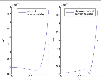
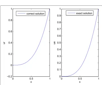
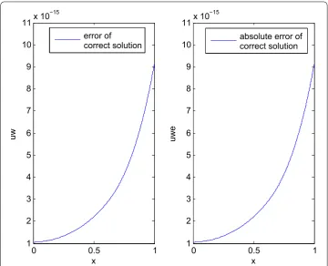
Whenn= 4, the absolute error is bigger, we do correction for the numerical solution withn= 4 and obtain the correct solution withn= 4,m= 8, the correct solution and the absolute error of correct solution are shown in Fig.7and Fig.8.

Figure 1The absolute error between the numerical solution and the exact solution withn= 4 for Example1

Figure 3The absolute error between the numerical solution and the exact solution withn= 7 for Example1

Table 1 The absolute errors withn= 4, 6, 7 for Example1

x The absolute errors withn= 4 The absolute errors withn= 6 The absolute errors withn= 7

0.2 0.0844 0.0044 2.81025203108243e–15

0.4 0.3501 0.0079 6.63358257213531e–15

0.6 0.6734 0.0143 3.27515792264421e–15

0.8 1.0234 0.0214 4.25770529943748e–14

1 1.6700 0.0280 2.43819897540083e–13

of convergencengets larger, the approximation between the numerical solution and the exact solution is better.

From Fig.1, Fig.7, Fig.8, we see that the absolute error of correct solution is smaller than the absolute error of numerical solution.

Example2 Consider the following multi-order fractional differential equation:

Dαu(x) =y0Dβ0_{u(x) +y1D}β1_{u(x) +y2D}β2_u(x)

+y3Dβ3_{u(x) +f(x), x}∈_{[0, 1],}

with the initial conditions

Figure 4The numerical solution and the exact solution withn= 6 for Example1

Figure 6The numerical solution and the exact solution withn= 8 for Example1

Figure 8The error of correct solution and the absolute error of correct solution withn= 4,m= 8 for Example1

whereα= 2,d0=d1= 0, the coefficient isy0=y2= –1,y1= 0,y3= 2, andβ0= 0,β2=2₃ ∈ (0, 1),β3=5₃∈(1, 2). The known function is

f(x) =x3+ 6x– 12

(7₃)x

4

3 ₊ 6

(10₃)x

7 3_,

the exact solution isu(x) =x3_.

Whenn= 2, the discrete variable isxi=₃i–1₆(i= 1, 2, 3), the numerical solution isu(x) =

CT

1(x), the unknown coefficient can be obtainedC1= [–0.0912, –0.0695, 0.0139]T, the shifted Chebyshev polynomials of approximation function(x) are

(x) = ⎡ ⎢ ⎣

1 2x– 1 8x2_{– 2x– 1}

⎤ ⎥ ⎦.

When n= 3, the discrete variable is xi= ₄i – 1₈(i= 1, 2, 3, 4), the numerical solution isu(x) =CT

1(x), the unknown coefficient can be obtainedC1= [0.3125, 0.4688, 0.1875, 0.0313]T_{, the shifted Chebyshev polynomials of approximation function(x) are}

(x) = ⎡ ⎢ ⎢ ⎢ ⎣

1 2x– 1 8x2– 2x– 1 32x3_{– 48x}2_{+ 18x– 1}

Whenn= 2, 3, the absolute errors for equation in some match points between the nu-merical solution and the exact solution are shown in Fig.9, Fig.10, and Table2. When

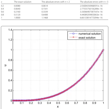
n= 3, 4, the numerical solution and the exact solution are shown in Fig.11, Fig.12.

Figure 9The absolute error between the numerical solution and the exact solution withn= 2 for Example2

Table 2 The absolute errors withn= 2, 3 for Example2

x The exact solution The absolute errors withn= 2 The absolute errors withn= 3

0.2 0.0080 0.0614 2.55004350968591e–16

0.4 0.0640 0.1541 2.77555756156289e–16

0.6 0.2160 0.3339 3.33066907387547e–16

0.8 0.5120 0.6488 4.44089209850063e–16

1 1.0000 1.1468 6.66133814775094e–16

Figure 11 The numerical solution and the exact solution withn= 3 for Example2

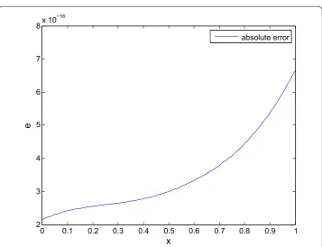
Whenn= 2, the absolute error is bigger, we do the correction for the numerical solution withn= 2 and obtain the correct solution withn= 2,m= 4, the correct solution and the absolute error of correct solution are shown in Fig.13, Fig.14.

The author of [32] researched the exact solution of Example2to obtain the absolute error of the correction solution, so that the accuracy of the numerical solution is improved. From Fig.9, Fig.10, and Table2, we see that, whenn= 2, the absolute error is bigger, when

n= 3, the absolute error becomes smaller and the precision of numerical solution is higher, the absolute error achieves about 10–16_{. From Fig.11, Fig.12, we see that, as the order of} convergencengets larger, the convergence effect between the numerical solution and the exact solution is better.

From Fig.9, Fig.13, Fig.14, it is seen that the absolute error of correct solution is clearly smaller.

8 Conclusion

frac-Figure 12 The numerical solution and the exact solution withn= 4 for Example2

Figure 14 The error of correct solution and the absolute error of correct solution withn= 2,m= 4 for Example2

tional differential operator matrix is deduced, but also this approach reduces the problem to a set of algebraic equations. We investigate multi-order fractional differential equation of error correction and analyze the convergence of the shifted Chebyshev polynomials. From example, it is seen that,nis bigger, the absolute error is smaller, and the conver-gence effect between the numerical solution and the exact solution is better. We do the correction for the numerical solution, the absolute error of correct solution is smaller than the absolute error of numerical solution. Numerical experiments are given to demonstrate the applicability of the method and the validity of error correction.

Acknowledgements

The authors would like to thank the referees for careful reading and several constructive comments and for making some useful corrections that have improved the presentation of the paper. The authors would like to thank the School of Science, Yanshan University, Qinhuangdao, Hebei, P.R. China for providing a good learning environment and INSA Centre Val de Loire, Université d’Orléans for offering to help.

Funding

This work is supported by the Natural Science Foundation of Hebei Province (A2017203100) in China and the LE STUDIUM RESEARCH PROFESSORSHIP award of Centre-Val de Loire region in France.

Availability of data and materials

Not applicable.

Competing interests

The authors declare that they have no competing interests.

Authors’ contributions

Author details

1_{School of Sciences, Yanshan University, Qinhuangdao, P.R. China.}2_{Loire Valley Institute for Advanced Studies, Orléans,}

France. 3_{PRISME (INSA-Institut National des Sciences Appliquées)-88, Bourges, France.}4_{INSA Centre Val de Loire,}

Université d’Orléans, Bourges, France.

Publisher’s Note

Springer Nature remains neutral with regard to jurisdictional claims in published maps and institutional affiliations.

Received: 28 January 2018 Accepted: 21 May 2018

References

1. Anastassiou, G.A., Argyros, I.K., Kumar, S.: Monotone convergence of extended iterative methods and fractional calculus with applications. Fundam. Inform.151(1–4), 241–253 (2017)

2. Hajipour, M., Jajarmi, A., Baleanu, D.: An efficient nonstandard finite difference scheme for a class of fractional chaotic systems. J. Comput. Nonlinear Dyn.13(2), 021013 (2017)

3. Jajarmi, A., Hajipour, M., Baleanu, D.: New aspects of the adaptive synchronization and hyperchaos suppression of a financial model. Chaos Solitons Fractals99, 285–296 (2017)

4. Baleanu, D., Jajarmi, A., Hajipour, M.: A new formulation of the fractional optimal control problems involving Mittag–Leffler nonsingular kernel. J. Optim. Theory Appl.175(3), 718–737 (2017)

5. Baleanu, D., Jajarmi, A., Asad, J.H., Blaszczyk, T.: The motion of a bead sliding on a wire in fractional sense. Acta Phys. Pol.131(6), 1561–1564 (2017)

6. Kumar, D., Singh, J., Baleanu, D.: A new analysis of Fornberg–Whitham equation pertaining to a fractional derivative with Mittag–Leffler type kernel. Eur. Phys. J. Plus133(2), 70 (2018).https://doi.org/10.1140/epjp/i2018-11934-y 7. Kumar, D., Singh, J., Baleanu, D.: Modified Kawahara equation within a fractional derivative with non-singular kernel.

Therm. Sci. (2017).https://doi.org/10.2298/TSCI160826008K

8. Singh, J., Kumar, D., Hammouch, Z., Atangana, A.: A fractional epidemiological model for computer viruses pertaining to a new fractional derivative. Appl. Math. Comput.316, 504–515 (2018)

9. Inc, M., Yusuf, A., Aliyu, A.I., Baleanu, D.: Soliton structures to some time-fractional nonlinear differential equations with conformable derivative. Opt. Quantum Electron.50, 20 (2018)

10. Zeng, S., Baleanu, D., Bai, Y., Wu, G.: Fractional differential equations of Caputo–Katugampola type and numerical solutions. Appl. Math. Comput.315, 549–554 (2017)

11. Ali, N., Shah, K., Baleanu, D., Arif, M., Khan, R.A.: Study of a class of arbitrary order differential equations by a coincidence degree method. Bound. Value Probl.2017(1), 111 (2017)

12. Kumar, D., Singh, J., Baleanu, D.: A new numerical algorithm for fractional Fitzhugh–Nagumo equation arising in transmission of nerve impulses. Nonlinear Dyn.91, 307–317 (2018)

13. Kumar, D., Agarwal, R.P., Singh, J.: A modified numerical scheme and convergence analysis for fractional model of Lienard’s equation. J. Comput. Appl. Math. (2017)http://doi.org/10.1016/j.cam.2017.03.011

14. Sakar, M.G., Akgül, A., Baleanu, D.: On solutions of fractional Riccati differential equations. Adv. Differ. Equ.2017(1), 39 (2017)

15. Jafarian, A., Mokhtarpour, M., Baleanu, D.: Artificial neural network approach for a class of fractional ordinary differential equation. Neural Comput. Appl.28(4), 765–773 (2017)

16. Jafari, H., Lia, A., Tejadodi, H., Baleanu, D.: Analysis of Riccati differential equations within a new fractional derivative without singular kernel. Fundam. Inform.151(1–4), 161–171 (2017)

17. Chen, Y.M., Han, X.N., Liu, L.C.: Numerical solution for a class of linear system of fractional differential equations by the Haar wavelet method and the convergence analysis. Comput. Model. Eng. Sci.97(5), 391–405 (2014)

18. Chen, Y.M., Sun, L., Liu, L.L., Xie, J.Q.: The Chebyshev wavelet method for solving fractional integral and differential equations of Bratu-type. J. Comput. Inf. Syst.9(14), 5601–5609 (2013)

19. Chen, Y.M., Sun, L., Li, X., Fu, X.H.: Numerical solution of nonlinear fractional integral differential equations by using the second kind Chebyshev wavelets. Comput. Model. Eng. Sci.90(5), 359–378 (2013)

20. Chen, Y.M., Liu, L.Q., Li, B.F., Sun, Y.N.: Numerical solution for the variable order linear cable equation with Bernstein polynomials. Appl. Math. Comput.238, 329–341 (2014)

21. Chen, Y.M., Sun, Y., Liu, L.Q.: Numerical solution of fractional partial differential equations with variable coefficients using generalized fractional-order Legendre functions. Appl. Math. Comput.244, 847–858 (2014)

22. Baleanu, D., Inc, M., Yusuf, A., Aliyu, A.I.: Space-time fractional Rosenou–Haynam equation: Lie symmetry analysis, explicit solutions and conservation laws. Adv. Differ. Equ.2018, 46 (2018)

23. Baleanu, D., Inc, M., Yusuf, A., Aliyu, A.I.: Time fractional third-order evolution equation: symmetry analysis, explicit solutions and conservation laws. J. Comput. Nonlinear Dyn.13, 021011 (2018)

24. Firoozjaee, M.A., Yousefi, S.A., Jafari, H., et al.: On a numerical approach to solve multi order fractional differential equations with boundary initial conditions. J. Comput. Nonlinear Dyn. (2015)

25. Aphithana, A., Ntouyas, S.K., Tariboon, J.: Existence and uniqueness of symmetric solutions for fractional differential equations with multi-order fractional integral conditions. Bound. Value Probl.2015(1), 1 (2015)

26. Hesameddini, E., Rahimi, A., Asadollahifard, E.: On the convergence of a new reliable algorithm for solving multi-order fractional differential equations. Commun. Nonlinear Sci. Numer. Simul.34, 154–164 (2016)

27. Dabiri, A., Butcher, E.A.: Stable fractional Chebyshev differentiation matrix for the numerical solution of multi-order fractional differential equations. Nonlinear Dyn.90(1), 185–201 (2017)

28. Saeedi, H.: A fractional-order operational method for numerical treatment of multi-order fractional partial differential equation with variable coefficients. SeMA J.7, 1–13 (2017)

29. Dabiri, A., Butcher, E.A.: Numerical solution of multi-order fractional differential equations with multiple delays via spectral collocation methods. Appl. Math. Model.56, 424–448 (2018)

31. Pimenov, V.G., Hendy, A.S.: Numerical studies for fractional functional differential equations with delay based on BDF-type shifted Chebyshev approximations. Abstr. Appl. Anal.2015(3), Article ID 510875 (2015)