R E S E A R C H
Open Access
Approximate solution of linear and
nonlinear fractional differential equations
under m-point local and nonlocal
boundary conditions
Hammad Khalil
1,2*, Rahmat Ali Khan
3, Dumitru Baleanu
4and Samir H Saker
5*Correspondence:
1Department of Mathematics,
University of Poonch Rawalakot, Rawalakot, 12350, Pakistan
2Department of Mathematics,
University of Malakand, P.O. Box 18000, Chakdara, Dir Lower, Khybarpukhtunkhwa, Pakistan Full list of author information is available at the end of the article
Abstract
This paper investigates a computational method to find an approximation to the solution of fractional differential equations subject to local and nonlocalm-point boundary conditions. The method that we will employ is a variant of the spectral method which is based on the normalized Bernstein polynomials and its operational matrices. Operational matrices that we will developed in this paper have the ability to convert fractional differential equations together with its nonlocal boundary
conditions to a system of easily solvable algebraic equations. Some test problems are presented to illustrate the efficiency, accuracy, and applicability of the proposed method.
MSC: 35C11; 65T99
Keywords: Bernstein polynomials; operational matrices;m-point boundary conditions; fractional differential equations
1 Introduction
Recently the studies of fractional differential equations (FDEs) gained the attention of many scientists around the globe. This topic remains a central point in several special issues and books. Fractional-order operators are nonlocal in nature and due to this prop-erty, they are most nicely applicable to various systems of natural and physical phenomena. This property has motivated many scientists to develop fractional-order models by con-sidering the ideas of fractional calculus. Examples of such systems can be found in many disciplines of science and engineering such as physics, biomathematics, chemistry, dy-namics of earthquakes, dynamical processes in porous media, material viscoelastic theory, and control theory of dynamical systems. Furthermore, the outcome of certain observa-tions indicates that fractional-order operators possess some properties related to systems having long memory. For details of applications and examples, we refer the reader to the work in [–].
The qualitative study of FDEs which discusses analytical investigation of certain prop-erties like existence and uniqueness of solutions has been considered by several authors. In Guptta [] studied the solvability of three point boundary value problems (BVPs).
Since then many researchers have been working in this area and provided many useful results which guarantee the solvability and existence of a unique solution of such prob-lems. For the reader interested in the existence theory of such problem we refer to work presented by Ruyun Ma [] in which the author presents a detailed survey on the topic. In [] the author derived an analytic relation which guarantees the existence of positive solution of a general third order multi-point BVPs. Also some analytic properties of so-lutions of FDEs are discussed by El-Sayed in []. Often it is impossible to arrive at the exact solution when FDEs has to be solved under some constraints in the form of bound-ary conditions. Therefore the development of approximation techniques remains a central and active area of research.
The spectral methods, which belong to the approximation techniques, are often used to find approximate solution of FDEs. The idea of the spectral method is to convert FDEs to a system of algebraic equations. However, different techniques are used for this con-version. Some of well-known techniques are the collocation method, the tau method, and the Galerkin method. The tau and Galerkin methods are analogous in the sense that the FDEs are enforced to satisfy some algebraic equations, then some supplementary set of equations are derived using the relations of boundary conditions (see,e.g., [] and the references therein). The collocation method [, ], which is an analog of the spectral method, consists of two steps. First, a discrete representation of the solution is chosen and then FDEs are discretized to obtain a system of algebraic equations.
These techniques are extensively used to solve many scientific problems. Dohaet al.[] used collocation methods and employed Chebyshev polynomials to find an approximate solution of initial value problems of FDEs. Similarly, Bhrawyet al.[] derived an explicit relation which relates the fractional-order derivatives of Legendre polynomials to its se-ries representation, and they used it to solve some scientific problems. Saadatmandi and Dehghan [] and Dohaet al.[] extended the operational matrices method and derived operational matrices of fractional derivatives for orthogonal polynomials and used it for solving different types of FDEs. Some recent and good results can be found in the articles like [, , ].
Some other methods have also been developed for the solution of FDEs. Among oth-ers, some of them are iterative techniques, reproducing kernel methods, finite difference methods etc. Esmaeili and Shamsi [] developed a new procedure for obtaining an ap-proximation to the solution of initial value problems of FDEs by employing a pseudo-spectral method, and Pedas and Tamme [] studied the application of spline functions for solving FDEs. In [], the author used a quadrature tau method for obtaining the nu-merical solution of multi-point boundary value problems. Also the authors in [–] ex-tended the spectral method to find a smooth approximation to various classes of FDEs and FPDEs. Some recent results in which orthogonal polynomials are applied to solve various scientific problems can be found in [–].
Bernstein polynomials are frequently used in many numerical methods. Bernstein poly-nomials enjoy many useful properties, but they lack the important property of orthogo-nality. As the orthogonality property is one of more important properties in approxima-tion theory and numerical simulaapproxima-tions, these polynomials cannot be directly implemented in the current technique of numerical approximations. To overcome this difficulty, these non-orthogonal Bernstein polynomials are transformed into an orthogonal basis [–]. But as the degree of the polynomials increases the transformation matrix becomes ill con-ditioned [, ], which results some inaccuracies in numerical computations. Recently Bellucci introduced an explicit relation for normalized Bernstein polynomials []. One applied Gram-Schmidt orthonormalization process to some sets of Bernstein polynomi-als of different scale levels, identifying the pattern of polynomipolynomi-als, and generalizing the result. The main results presented in this article are based on these generalized bases.
In this article we present an approximation procedure to find an approximate solution of the FDEs subject to local and nonlocalm-point BVPs. The method is designed to solve lin-ear FDEs with constant coefficients, linlin-ear FDEs with variable coefficients, and nonlinlin-ear FDEs, under local and nonlocalm-point boundary conditions. In particular, we consider the following generalized class of FDEs:
DσU(t) = p
i=
λiDρiU(t) +f(t), ()
DσU(t) =
p
i=
λi(t)DρiU(t) +f(t), ()
DσU(t) +
p
i=
λiDρiU(t) =FU(t)ρ,U(t)ρ, . . . ,U(t)ρp+f(t). ()
In equation ()λi∈R,t∈[,ω],f(t)∈C([,ω]). The orders of the derivatives are defined
as
<ρ≤ <ρ≤· · ·p– <ρp≤p<σ≤p+ .
In equation ()λi(t)∈C([,ω]). In ()F(U(t)ρ,U(t)ρ, . . . ,U(t)ρp) is a nonlinear function
ofU(t) and its fractional derivatives.
The main aim in this paper is to find a smooth approximation toU(t), which satisfies a given set ofm-point boundary conditions. We consider the following two types of bound-ary constraints.
Type :Multi-point local boundary conditions defined as
U() =u, U(τi) =ui, i= , ,p– , U(ω) =up. ()
Type :Non localm-point boundary conditions, defined as
Uj() =uj, j= , , . . . ,p– , ˆ
m–
i=
We use the normalized Bernstein polynomials for our investigation, which is based on the explicit relations presented in []. We use these polynomials to develop new operational matrices. We develop four operational matrices, two of them being operational matrices of integration and differentiation, the formulation technique for these two operational matrices is the same as that used for traditional orthogonal polynomials. We introduce two more operational matrices to deal with the local and nonlocal boundary conditions. To the best of our knowledge such types of operational matrices are not designed for normalized Bernstein polynomials.
We organized the rest of article as follows. In Section , we recall some basic concepts definition from fractional calculus, approximation theory, and matrix theory. Also we present some properties of normalized Bernstein polynomials which are helpful in our further investigation. In Section , we present a detailed procedure for the construction of the required operational matrices. In Section , the developed matrices are employed to solve FDEs by introducing a new algorithm. In Section , the proposed algorithm is applied to some test problems to show the efficiency of the proposed algorithm. The last section is devoted to a short conclusion.
2 Some basic definitions
In this section, we present some basic notation and definitions from fractional calculus and well-known results which are important for our further investigation. More details can be found in [, ].
Definition The Riemann-Liouville fractional-order integral of orderσ∈R+of a
func-tionφ(t)∈(L[a,b], R) is defined by
aItσφ(t) = (σ)
t
a
(t–s)σ–φ(s)ds. ()
The integral on right hand side exists and is assumed to be convergent.
Definition For a given functionφ(t)∈Cn[a,b], the fractional-order derivative in the
Caputo sense, of orderσis defined as
Dσφ(t) =
(n–σ)
t
a
φ(n)(s)
(t–s)σ+–nds, n– ≤σ<n,n∈N.
The right side is assumed to be point wise defined on (a,∞), wheren= [σ] + in the case thatσ is not an integer.
This leads toIσtk= (+k) (+k+σ)t
k+σ forσ> ,k≥,DσC= , for a constantCand
Dσtk= ( +k)
( +k–σ)t
k–σ, fork≥[σ]. ()
Throughout the paper, we will use the Brenstein polynomials of degreen. The analytic relation of the Brenstein polynomials of degreendefined on [, ] is given as
B(i,n)(t) =
n–i
k=
(–)k
n i
n–i k
The set of polynomials defined by () have a lot of interesting properties. They are posi-tive on [, ] and also approximate a smooth function on the domain [, ]. The polynomi-als defined in () are not orthogonal, after the application of the Gram-Schmidt process the explicit form of normalized Bernstein polynomials is obtained (as discussed in detail in []) by
φj,n(t) =(n–j) + ( –t)n–j
j
k=
(j,k)tj–k, ()
where
(j,k)= (–)k
(n–k+ ) (j– )
(j–k+ ) (n–j+ ) (k+ ) (j–k+ ).
The polynomials defined in () are not directly applicable in construction of operational matrices (it will be clear in the next section). Therefore, we further generalize the relation
φj,n(t) =(n–j) +
j
k=
n–j
l=
(j,k,l)tl+j–k, ()
where
(j,k,l)=
((–)(n–j+k+l) (n–j+ ) (n–k+ ) (j+ ))
(l+ ) (n–j–l+ ) (j–k+ ) (n–j+ ) (k+ ) (j–k+ ). ()
Note that in equation (),φj,n(t) is of degreenfor all choices ofj. By analyzing we observe that the minimum power oftis at maximum value ofkand minimum value ofl, which is . Conversely the maximum power oftisn. These polynomials are orthogonal on the interval [, ]. To make them applicable on the interval [,ω], we simply make substitution oft=ωt without loss of generality. So we can write the orthogonal Bernstein polynomials on the interval [,ω] as follows:
φj,n(t) = w(j,n)
j
k=
n–j
l=
(j,k,l)
tl+j–k
ωl+j–k, ()
where w(j,n)=
(n–j) + /√ω. The orthogonality relation for these polynomials is de-fined as follows:
ω
φi,n(t)φj,n(t) =δ(i,j). ()
As usual we can approximate any functionf∈C[,ω] in the normalized Bernstein poly-nomial as
f(t) =
n
j=
cjφj,n(t), wherecj=
ω
f(t)φj,n(t)dt, ()
which can always be written as
f(t) = HTN
ω
where HT
Nand
ω
N(t) are N =n+ terms column vector containing coefficients and Bern-stein polynomials, respectively, and one defined
HTN= [c,c, . . . ,cn], ()
ω
N(t) =
φ,n(t),φ,n(t), . . . ,φj,n(t)T. ()
As N represents the size of the resulting algebraic equations it is considered as a scale level of the scheme.
The integral of the triple product of fractional-order Legendre polynomials over the do-main of interest was recently used in []. There the author used this value to solve frac-tional differential equations with variable coefficients directly. We use a triple product for Bernstein polynomials to construct a new operational matrix which is of basic importance in solving FDEs with variable coefficients. The following theorem is of basic importance.
Theorem The definite integral of the product of three Bernstein polynomials over the domain[,ω]is constant and is defined as
ω
Proof Consider the following expression:
ω
Theorem [, ] Consider a matrix V defined as
3 Operational matrices of derivative and integral
Now we are in a position to construct new operational matrices. The operational matrices of derivatives and integrals are frequently used in the literature to solve fractional-order differential equations. In this section, we present the proofs of constructions of four new operational matrices. These matrices act as building blocks in the proposed method.
Theorem The fractional integration of orderσ of the function vectorωN(t) (as defined
in())is defined as
whereP((σN,ω×)N)is an operational matrix for fractional-order integration and is given as
Proof Consider the general element of () and apply fractional integral of orderσ, con-sequently we will get
Iσφr,n(t) = w(r,n)
Using the definition of fractional-order integration we may write
Iσφr,n(t) = w(r,n)
σ with normalized
Bern-stein polynomials as follows:
tl+r–k+σ =
Using equation (), we can write
c(r,s)= w(s,n)
On further simplifications, we can get
c(r,s)= w(s,n)
whereD((σN,×ω)N)is defined as
Proof On application of the derivative of orderσ to a general element of (), we may write
Using the definition of the fractional-order derivative we can easily write
Dσφr,n(t) = w(r,n)
We can approximatetl+r–k–σ with the Bernstein polynomials as follows:
tl+r–k–σ=
Using equation (), we can write
On further simplification we can get
The operational matrices developed in the previous theorems can easily solve FDEs with initial conditions. Here we are interested in the approximate solution of FDEs under com-plicated types of boundary conditions. Therefore we need some more operational matrices such that we can easily handle the boundary conditions effectively.
The following matrix plays an important role in the numerical simulation of fractional differential equations with variable coefficients.
Theorem For a given function f ∈C[,ω],and u= HT
N
ω
N(t),the product of f(t)andσ
order fractional derivative of the function u(t)can be written in matrix form as
Proof Applying Theorem we can write
Dσu(t) = HTND
(σ,ω) (N×N)
ω
N(t) ()
and
f(t)Dσu(t) = HT ND
(σ,ω) (N×N)
ω
N(t), ()
where
ω
N(t) =
f(t)φ,n(t),f(t)φ,n(t), . . . ,f(t)φn,n(t)T.
Consider the general element of ωN(t), and approximate it with normalized Bernstein polynomials as
f(t)φr,n(t) =
n
s=
crsφs,n(t), ()
wherecri can easily be calculated as
crs=
ω
f(t)φr,n(t)φs,n(t)dt. ()
Now asf(t)∈C[,ω], we can approximate it with normalized Bernstein polynomials as
f(t) =
n
q=
dqφq,n(t),
dq=
ω
f(t)φq,n(t)dt.
()
Using equation () in () we get the following estimates:
crs=
n
q=
dq ω
φq,n(t)φr,n(t)φs,n(t)dt. ()
In view of Theorem we obtain the following estimate:
crs=
n
q=
dq(q,r,s). ()
Using () in ()
f(t)φr,n(t) =
n
s=
n
q=
Evaluating () fors= , , . . . ,nandr= , , . . . ,nwe can write
Using () in () we get the desired result. The proof is complete.
Since one of our aims in this paper is to solve FDEs under different types of local and non-local boundary conditions, we have to face some complicated situations, so to handle these situations we will use the operational matrix developed in the next theorem.
Theorem Let f be a function of the form f(t) =atn where a∈Rand n∈N,then for
The entries of the matrix are defined by
(i,j)=a(i,σ,τ,ω)w(j,n)
Using () we may write
can be approximated with Bernstein polynomials as follows:
a(i,σ,τ,ω)tn
proof is complete.
4 Application of operational matrices
The operational matrices derived in the previous section play a central role in the nu-merical simulation of FDEs under different types of boundary conditions. We start our discussion with the following class of FDEs:
The solution to this equation can be assumed in terms of series representation of normal-ized Bernstein polynomials such that the following relation holds:
DσU(t) = HTN
ω
N(t). ()
Now by the application of fractional integral of orderσ, and use of Theorem , we can explicitly writeU(t) as follows:
U(t) –
N, which is an unknown vector. We will use this vector to get the solution to the problem.
Type :Suppose we have to solve () under the following condition:
U() =u, U(τi) =ui, i= , ,p– , U(ω) =up, ()
ccan easily be obtained using the initial conditionU() = . The solution in () must
satisfy all the conditions, therefore using the conditions at the intermediate and boundary points we have
In order to make the notation simple we useτp=ωin last equation. Equation () can
then also be written in matrix form as
The matrix in the left is a Vandermonde matrix, in view of Theorem its inverse exists. Using the inverse ofVwe get the values ofci:
ci=
Using the values ofciin equation () we may write
U(t) –u–
In simplified notation we can write
U(t) –g(t) + of Theorem , we can easily get
U(t) + HTN
In simplified notation we can write
U(t) = HTNEN×N
isN×Nmatrix related to type boundary conditions. For instance we stop the current procedure here and discuss the procedure of obtaining analogous relation forU(t) under type boundary conditions.
Type :Suppose if we need to solve the problem underm-point non-local boundary conditions
However, the last constantcpis unknown. In order to get a relation forcpwe use nonlocal boundary conditions. Using them-point boundary condition we get
U(ω) = HT
From (), we see that left sides of () and () are equal, therefore for the sake of ob-taining the value ofcp, we can write
On further simplification we get
cp=
N(t). On further simplification we can write
We see that for both local and non-local boundary conditions we getU(t) in matrix form ary conditions are given, otherwise useE=E. Now using () and using Theorem , we can write
After a long calculation and simplification we get
HTN– HTNEN×N
We see that () is an easily solvable matrix equation and it can easily be solved for HTN, by using HT
Nin () this will lead us to an approximate solution to the problem. Next, we consider the linear FDEs with variable coefficients,
DσU(t) =
Using the integral of orderσwe can write
U(t) = HTN
Approximatingf(t) = FT
N
ω
N(t), and using (), () in () we may write
HTNωN(t) = HTNEN×N p
i=
Q(λi(t),ρi,ω) (N×N)
ω
N(t)
+ GTN
p
i=
Q(λi(t),ρi,ω)
(N×N)
ω
N(t) + F T
N
ω
N(t). ()
On rearranging we get
HTN– HTNEN×N p
i=
Q(λi(t),ρi,ω)
(N×N) + G
T N
p
i=
Q(λi(t),ρi,ω)
(N×N) – F
T
N= . ()
Now, we consider the nonlinear FDEs. The nonlinear FDEs are often very difficult to solve with operational matrix techniques. One way is to use the collocation method, by doing so the FDEs result in nonlinear algebraic equations. These nonlinear algebraic equa-tions are then solved iteratively using the Newton method or some other iterative method. The second approach is to linearize the nonlinear part of the fractional differential equa-tion using a quasilinearizaequa-tion technique. Doing so the nonlinear fracequa-tional differential equations is converted to a recursively solvable linear differential equations. This tech-nique was introduced recently and has been used to find an approximate solution of many scientific problem. The quasilinearization method was introduced by Bellman and Kalaba [] to solve nonlinear ordinary or partial differential equations as a generalization of the Newton-Raphson method. The origin of this method lies in the theory of dynamic pro-gramming. In this method, the nonlinear equations are expressed as a sequence of linear equations and these equations are solved recursively. The main advantage of this method is that it converges monotonically and quadratically to the exact solution of the original equations []. Also some other interesting work in which quasilinearization method is applied to scientific problems is in [–]. Consider a nonlinear fractional-order differ-ential equation of the form
DσU(t) + p
i=
λiDρiU(t) =F
U(t)ρ,U(t)ρ, . . . ,U(t)ρp+f(t). ()
The general procedure of this method is as given now. First solve the linear part with a given set of local or nonlocal conditions
DσU(t) + p
j=
λiDρiU(t) =f(t). ()
The next step is to linearize the nonlinear part with a multivariate Taylor series expan-sion aboutU(t). So after linearizing and simplification we get
DσU()(t) +
p
j=
λjDρjU
()(t)
=F(U()(t),U()γ(t),U
ρ
()(t), . . . ,U
ρn
()(t)
+
n
j=
U()ρj –Uρi
()
∂f
∂Uρj
U()(t),U()ρ(t),U
ρ
()(t), . . . ,U
ρn
()(t)
+f(t).
()
The above equation is an FDE with variable coefficients. It can easily be solved with the method developed in Section .. The solution at this stage will be labeledU(t) and is
the solution of the problem at first iteration. Again we have to linearize the problem about
U(t) to obtain the solution at second iteration. The whole process can be seen as a
recur-rence relation like
DσU(r+)(t) +
n
j=
bj(t)DρjU
(r+)(t) =F(t) .
And the boundary conditions become
Urj+() =uj, Ur+(τ) =
m–
i=
ζiUr+(ηi),
wherebj(t) =λj–∂U∂fρj(U(r)(t),U(ρr)(t),U
ρ
(r)(t), . . . ,U
ρn
(r)(t)) and
F(t) =fU(r)(t),U(ρr)(t),U(ρr)(t), . . . ,U(ρrn)(t)
–
n
j=
U(ρrj) ∂f
∂Uρj +g(t).
It can be easily noted that the above equation is fractional differential equation with vari-able coefficients. Using the initial solutionX(t) we may start the iterations. The
coeffi-cientsbi(t) and the source termF(t) can be updated at every iterationrto get the next solution atr+ . At every step we may solve the problem at given nonlocal boundary con-ditions. We assume that the method converges to the exact solution of the problem if there is convergence at all.
5 Examples
To show the applicability and efficiency of the proposed method, we solve some fractional differential equations. The numerical simulation is carried out usingMatLab. However, we believe that the algorithm can be simulated using any simulation tool kit.
Example As a first problem we solve the following linear integer order boundary value problem
DU(t) = D
U(t) +
DU(t) +
where
g(t) =
%
&
·πsin(πt) –πcos(πt) – sin(πt) + πsin(πt).
We can easily see that the exact solution isU(t) =sin(πt). We test our algorithm by solving this problem under the following sets of boundary conditions:
S=
'
U() = ,U %
&
= .,U %
&
= –,U() =
(
,
S=
!
U() = ,U(.) = ,U(.) = ,U() = ",
S=
!
U() = ,U() =π,U() = ,
U() + .U(.) +U(.) + .U(.) + .U(.) =U()".
We approximate the solution to this problem with different types of boundary conditions and observe that the approximate solution is very accurate. For illustration purposes we calculate the absolute difference at a different scale levels. The results are displayed in Figure and Figure for boundary conditionsS andS, respectively. We compare the
exact solution and approximate solution under boundary conditionsSat different scale
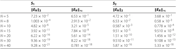
levels, and the results are displayed in Table . It can easily be noted that with increase of scale level, that the approximate solution becomes more and more accurate, and at scale levelN= , the approximate solution is accurate up to the seventh digit. The accuracy may be increased by using a high scale level. For instance we simulate the algorithm at high scale level and measure EN and EN ∞at each scale levelN. Table shows these results at high scale levels under boundary conditionsS andS. From this example, we
conclude that the proposed method is convergent for integer order differential equations (linear).
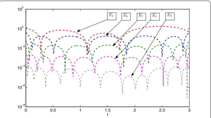
Figure 2 Absolute difference of exact and approximate solution for different values ofNunder boundary conditionS2.Here we fixω= 3, and use the notationEN=|Uexact–UN|.
Table 1 Comparison of exact and approximate solution of Example 1 using the boundary condition as defined inS
t N
ExactU(t) N = 5 N = 7 N = 9 N = 11
t= 0.4 0.95105651629 0.9677391807 0.9499276887 0.9510565133 0.95105651554
t= 0.8 0.58778525229 0.5806739865 0.5877691649 0.5877785192 0.5877882463
t= 1.2 –0.58778525229 –0.5879798137 –0.5877896195 –0.5877852801 –0.58778528235
t= 1.6 –0.95105651629 –0.9318025727 –0.9510687377 –0.9510565637 –0.9510565256
t= 2.0 –0.00000000000 –0.0160927142 –0.0000151536 –0.0000001456 –0.00000000975
t= 2.4 0.95105651629 0.9684572120 0.9510519403 0.9510565108 0.95105651183
t= 2.8 0.58778525229 0.5667990904 0.5879771600 0.5877852533 0.5877852523
t= 3 0.00000000000 0.0634719308 –0.0001774663 0.0000000045 0.00000000125
Table 2 Comparison of exact and approximate solution of Example 1 using the boundary condition as defined inS
S1 S2
EN2 EN∞ EN2 EN∞
N= 5 7.23×10⁻² 6.53×10⁻¹ 4.72×10⁻¹ 3.68×10⁻¹
N= 8 1.003×10⁻⁴ 2.913×10⁻² 6.53×10⁻² 0.58×10⁻³
N= 10 4.82×10⁻⁶ 3.21×10⁻⁵ 0.587×10⁻³ 0.778×10⁻⁴
N= 15 3.92×10⁻¹¹ 7.84×10⁻⁹ 9.51×10⁻⁵ 9.510×10⁻⁸
N= 20 6.22×10⁻¹⁶ 5.61×10⁻¹⁴ 1.51×10⁻¹⁰ 1.456×10⁻¹²
N= 30 9.36×10⁻¹⁹ 8.22×10⁻¹⁸ 9.510×10⁻¹¹ 9.108×10⁻¹³
N= 40 9.28×10⁻²¹ 0.781×10⁻¹⁸ 5.87×10⁻¹⁶ 5.33×10⁻¹⁸
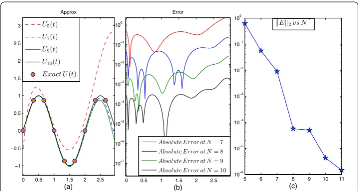
To show the efficiency of proposed method in solving nonlocal m-point boundary prob-lem, we solve Example under a -point nonlocal boundary condition as defined inS. We
observe that the method works well, the absolute difference is much less than –, a very
high accuracy for such complicated problems. We compare the approximate solution with the exact solution at different scale levels. We also calculate E at different scale levels.
Figure 3 Simulation and observation of Example 1. (a)Comparison of approximate solution at different scale levels with the exact solution.(b)Absolute difference of exact and approximate solution.
(c)Convergence of E 2at different scale levels.
Example As a second example consider the following fractional-order differential equa-tion:
D.U(t) +D.U(t) +D.U(t) +U(t) =g(t). () Here we considerg(t) as
g(t) = ,,,,,t
(t– ,t+ ,t– ,)
,,,,, –t
(t– )
–,,,,,t(,,t– ,,t + ,,t– ,,t+ ,,)
/,,,,,,,
–,,,,,t(,t– ,,t+ ,,t – ,,t+ ,,)/,,,,,,,. ()
We consider the following two types of boundary conditions:
S=
!
U() = ,U(.) = .,U(.) = .,U() = ",
S=
!
U() = ,U() = ,U() = ,
U() + .U(.) +U(.) + .U(.) – .U(.) =U()".
It can easily be observed that the exact solution of the problem isU(t) =t(t– ).
We solve this problem with the proposed method under boundary conditionsS, and we
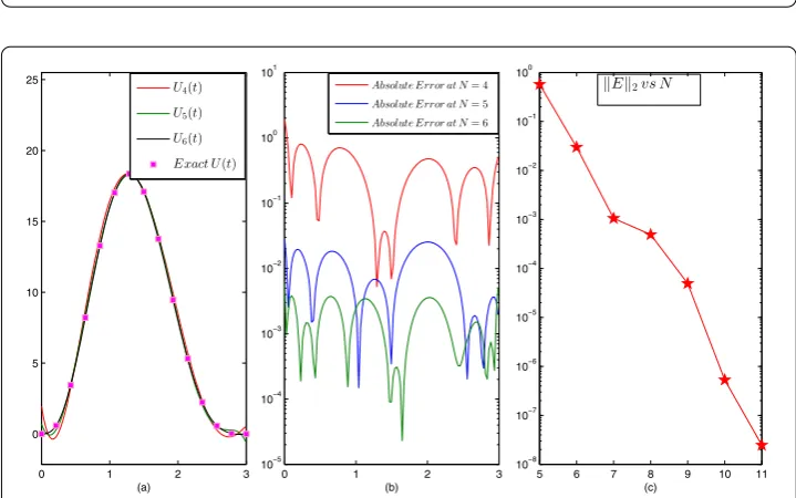
Figure 4 Example 2. (a)Comparison of approximate solution with the exact solution under boundary conditionS.(b)Absolute error obtained with the new method at different scale levels.(c) E 2obtained with the new method at different values ofN.
Figure 5 Example 2. (a)Comparison of approximate solution with the exact solution under boundary conditionS.(b)Absolute error obtained with the new method at different scale levels.(c) E 2obtained with the new method at different values ofN.
N= . We measure E at different values ofNand observe that the method is highly
convergent. We also approximate solution of this problem under boundary condition S. The results are displayed in Figure . We can easily observe that the approximate solution of the method converges to the exact solution as the value ofNincreases.
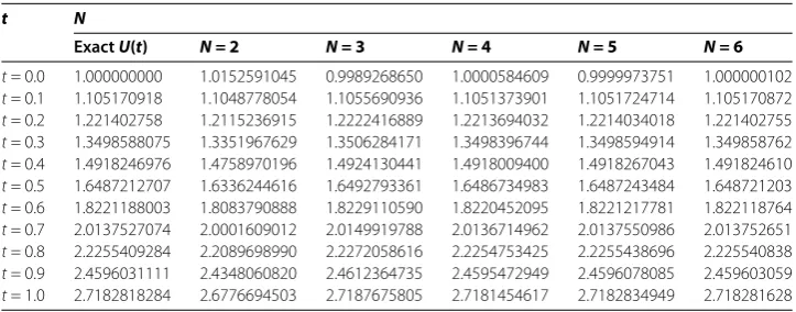
Example As a third example consider the following fractional differential equation with variable coefficients:
We consider the following types of boundary conditions:
S=
!
U() = ,U() = ,U(.) + .U(.) +U(.) – .U(.) =U()",
S=
!
U() = ,U(.) = .,U() = .".
We select a suitableg(t), such that the exact solution of the problem iset. We simulate the
proposed algorithm to solve this problem under boundary conditionsSand we observe
that the method works well. The results are displayed in Figure . In this figure we display the comparison of the exact and the approximate solution, the absolute error of approxi-mation and the square norm of the error. One can easily conclude that the method is highly efficient. We solve the problem under boundary conditionSand the results are displayed
in Table . One can easily see that the approximate solution is much more accurate.
Figure 6 Example 3. (a)Comparison of the approximate solution with the exact solution under boundary conditionS.(b)Absolute error obtained with the new method at different scale levels.(c) E 2obtained with the new method at different values ofN.
Table 3 Comparison of exact and approximate solution of Example 3 using the boundary condition as defined inS
t N
ExactU(t) N = 2 N = 3 N = 4 N = 5 N = 6
t= 0.0 1.000000000 1.0152591045 0.9989268650 1.0000584609 0.9999973751 1.000000102
t= 0.1 1.105170918 1.1048778054 1.1055690936 1.1051373901 1.1051724714 1.105170872
t= 0.2 1.221402758 1.2115236915 1.2222416889 1.2213694032 1.2214034018 1.221402755
t= 0.3 1.3498588075 1.3351967629 1.3506284171 1.3498396744 1.3498594914 1.349858762
t= 0.4 1.4918246976 1.4758970196 1.4924130441 1.4918009400 1.4918267043 1.491824610
t= 0.5 1.6487212707 1.6336244616 1.6492793361 1.6486734983 1.6487243484 1.648721203
t= 0.6 1.8221188003 1.8083790888 1.8229110590 1.8220452095 1.8221217781 1.822118764
t= 0.7 2.0137527074 2.0001609012 2.0149919788 2.0136714962 2.0137550986 2.013752651
t= 0.8 2.2255409284 2.2089698990 2.2272058616 2.2254753425 2.2255438696 2.225540838
t= 0.9 2.4596031111 2.4348060820 2.4612364735 2.4595472949 2.4596078085 2.459603059
Figure 7 Example 2,E2vs. iteration, for Example 4, obtained with the new method at different
values ofN. Here we use boundary conditionsS1.
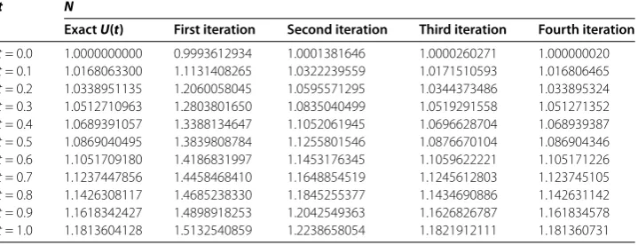
Example As a last example consider the following nonlinear fractional differential equation:
D.U(t) +D.U(t) +U(t) =D.UU+U+D.U+g(t), ()
with boundary conditions
S=
!
U() = ,U(.) = .,U() = .",
S=
'
U() = ,U() = ,
.U %
&
+ .U %
&
+ .U %
&
– .U %
&
=U()
(
.
Select a suitableg(t) such that the exact and unique solution of the above problem is
U(t) =et/. We approximate the solution of this problem with the iterative method
pro-posed in the paper under boundary conditionS. We carry out the iteration at different
scale levelsN. We observe that the method converges more rapidly to the exact solution for high values ofN. For instance, at some values ofNwe calculate E at each iteration.
The results are displayed in Figure , one can see that E falls below –at the fifth
iteration using scale levelN= . On solving the problem under boundary conditionsS
we observe that the method provides very accurate estimate of solution. The results are displayed in Table .
6 Conclusion
Table 4 Comparison of exact and approximate solution of Example 4 using the boundary condition as defined inS
t N
ExactU(t) First iteration Second iteration Third iteration Fourth iteration
t= 0.0 1.0000000000 0.9993612934 1.0001381646 1.0000260271 1.000000020
t= 0.1 1.0168063300 1.1131408265 1.0322239559 1.0171510593 1.016806465
t= 0.2 1.0338951135 1.2060058045 1.0595571295 1.0344373486 1.033895324
t= 0.3 1.0512710963 1.2803801650 1.0835040499 1.0519291558 1.051271352
t= 0.4 1.0689391057 1.3388134647 1.1052061945 1.0696628704 1.068939387
t= 0.5 1.0869040495 1.3839808784 1.1255801546 1.0876670104 1.086904346
t= 0.6 1.1051709180 1.4186831997 1.1453176345 1.1059622221 1.105171226
t= 0.7 1.1237447856 1.4458468410 1.1648854519 1.1245612803 1.123745105
t= 0.8 1.1426308117 1.4685238330 1.1845255377 1.1434690886 1.142631142
t= 0.9 1.1618342427 1.4898918253 1.2042549363 1.1626826787 1.161834578
t= 1.0 1.1813604128 1.5132540859 1.2238658054 1.1821912111 1.181360731
local and nonlocal boundary value problems. We use normalized Bernstein polynomi-als for our analysis. But the method can be used to generalize such types of operational matrices for almost all types of orthogonal polynomials. It is also possible to get a more approximate solution of such problems using other types of orthogonal polynomials like Legendre, Jacobi, Laguerre, Hermite etc. It is not clear to us which is the best set of or-thogonal polynomials for this method. Further investigation is required to generalize the method to solve other types of scientific problems.
Competing interests
The authors declare that they have no competing interests.
Authors’ contributions
The authors have made equal contributions in preparing the proofs and numerical simulations. The authors have approved the final manuscript.
Author details
1Department of Mathematics, University of Poonch Rawalakot, Rawalakot, 12350, Pakistan.2Department of Mathematics,
University of Malakand, P.O. Box 18000, Chakdara, Dir Lower, Khybarpukhtunkhwa, Pakistan.3Dean Faculty of Science,
University of Malakand, Chakdara, Dir Lower, Khybarpukhtunkhwa, Pakistan. 4Department of Mathematics and Computer
Science, Cankaya University, Ankara, Turkey. 5Department of Mathematics, Mansoura University, Al Mansurah, Muhafazat
ad Daqahliyah, Egypt.
Acknowledgements
The authors are thankful to the reviewers and the editor for carefully reading and useful suggestion which improved the quality of the article.
Received: 11 April 2016 Accepted: 24 June 2016
References
1. Baleanu, D, Diethelm, K, Scalas, E, Trujillo, JJ: Fractional Calculus Models and Numerical Methods, Series on Complexity, Nonlinearity and Chaos. World Scientific, Boston (2012)
2. Kilbas, AA, Srivastava, HM, Trujillo, JJ: Theory and Applications of Fractional Differential Equations. North-Holland Mathematics Studies, vol. 204. Elsevier, Amsterdam (2006)
3. Lazarevic, MP, Spasic, AM: Finite-time stability analysis of fractional order time-delay systems: Gronwall’s approach. Math. Comput. Model.49(3), 475-481 (2009)
4. Magin, RL: Fractional Calculus in Bioengineering. Begell House, Redding (2006) 5. Podlubny, I: Fractional Differential Equations. Academic Press, San Diego (1999)
6. Sabatier, J, Agrawal, OP, Machado, JAT (eds.): Advances in Fractional Calculus: Theoretical Developments and Applications in Physics and Engineering. Springer, Dordrecht (2007)
7. Zaslavsky, GM: Hamiltonian Chaos and Fractional Dynamics. Oxford University Press, Oxford (2008)
8. Gupta, CP: Solvability of a three-point nonlinear boundary value problem for a second order ordinary differential equation. J. Math. Anal. Appl.168, 540-551 (1992)
9. Ma, R: A survey on nonlocal boundary value problems. Appl. Math. E-Notes7, 257-279 (2007)
10. Guezane-Lakoud, A, Zenkoufi, L: Existence of positive solutions for a third-order multi-point boundary value problem. Appl. Math.3, 1008-1013 (2012)
12. Canuto, C, Hussaini, MY, Quarteroni, A, Zang, TA: Spectral Methods in Fluid Dynamics. Springer, New York (1988) 13. Bhrawy, AH, Alofi, AS: A Jacobi-Gauss collocation method for solving nonlinear Lane-Emden type equations.
Commun. Nonlinear Sci. Numer. Simul.17, 62-70 (2012)
14. Funaro, D: Polynomial Approximation of Differential Equations. Lecturer Notes in Physics. Springer, Berlin (1992) 15. Doha, EH, Bhrawy, AH, Ezz-Eldien, SS: Efficient Chebyshev spectral methods for solving multi-term fractional orders
differential equations. Appl. Math. Model.35, 5662-5672 (2011)
16. Bhrawy, AH, Alofi, AS, Ezz-Eldien, SS: A quadrature tau method for variable coefficients fractional differential equations. Appl. Math. Lett.24, 2146-2152 (2011)
17. Saadatmandi, A, Dehghan, M: A new operational matrix for solving fractional-order differential equations. Comput. Math. Appl.59, 1326-1336 (2010)
18. Doha, EH, Bhrawy, AH, Ezz-Eldien, SS: A Chebyshev spectral method based on operational matrix for initial and boundary value problems of fractional order. Comput. Math. Appl.62, 2364-2373 (2011)
19. Ghoreishi, F, Yazdani, S: An extension of the spectral Tau method for numerical solution of multi-order fractional differential equations with convergence analysis. Comput. Math. Appl.61, 30-43 (2011)
20. Vanani, SK, Aminataei, A: A Tau approximate solution of fractional partial differential equations. Comput. Math. Appl. 62, 1075-1083 (2011)
21. Esmaeili, S, Shamsi, M: A pseudo-spectral scheme for the approximate solution of a family of fractional differential equations. Commun. Nonlinear Sci. Numer. Simul.16, 3646-3654 (2011)
22. Pedas, AA, Tamme, E: On the convergence of spline collocation methods for solving fractional differential equations. J. Comput. Appl. Math.235, 3502-3514 (2011)
23. Bhrawy, AH, Al-Shomrani, MM: A shifted Legendre spectral method for fractional-order multi-point boundary value problems. Adv. Differ. Equ.20128 (2012)
24. Khalil, H, Khan, RA: The use of Jacobi polynomials in the numerical solution of coupled system of fractional differential equations. Int. J. Comput. Math. (2014). doi:10.1080/00207160.2014.945919
25. Shah, K, Ali, A, Khan, RA: Numerical solutions of fractional order system of Bagley-Torvik equation using operational matrices. Sindh Univ. Res. J. (Sci. Ser.)47(4), 757-762 (2015)
26. Khalil, H, Khan, RA: A new method based on Legendre polynomials for solutions of the fractional two-dimensional heat conduction equation. Comput. Math. Appl. (2014). doi:10.1016/j.camwa.2014.03.008
27. Khalil, H, Khan, RA: New operational matrix of integration and coupled system of Fredholm integral equations. Chin. J. Math.2014, Article ID 146013 (2014).
28. Khalil, H, Khan, RA: A new method based on Legendre polynomials for solution of system of fractional order partial differential equation. Int. J. Comput. Math.91, 2554-2567 (2014). doi:10.1080/00207160.2014.880781
29. Khalil, H, Khan, RA, Al Smadi, MH, Freihat, A: Approximation of solution of time fractional order three-dimensional heat conduction problems with Jacobi polynomials. J. Math.47(1), 35-56 (2015)
30. Khalil, H, Rashidi, MM, Khan, RA: Application of fractional order Legendre polynomials: a new procedure for solution of linear and nonlinear fractional differential equations under m-point nonlocal boundary conditions. Commun. Numer. Anal.2016(2), 144-166 (2016)
31. Khalil, H, Khan, RA, Baleanu, D, Rashidi, MM: Some new operational matrices and its application to fractional order Poisson equations with integral type boundary constrains. Comput. Appl. Math. (2016).
doi:10.1016/j.camwa.2016.04.014
32. Bhrawy, AH, Zaky, MA: A method based on the Jacobi tau approximation for solving multi-term time-space fractional partial differential equations. J. Comp. Physiol.281, 876-895 (2015)
33. Bhrawy, AH, Zaky, MA: Numerical simulation for two-dimensional variable-order fractional nonlinear cable equation. Nonlinear Dyn.80(1-2), 101-116 (2015)
34. Bhrawy, AH, Zaky, MA: New numerical approximations for space-time fractional Burgers’ equations via a Legendre spectral-collocation method. Rom. Rep. Phys.67(2), 340-349 (2015)
35. Zaky, MA, Bhrawy, AH, Van Gorder, RA: A space-time Legendre spectral tau method for the two-sided space-time Caputo fractional diffusion-wave equation. Numer. Algorithms71(1), 151-180 (2016)
36. Bhrawy, AH, Zaky, M: Shifted fractional-order Jacobi orthogonal functions: application to a system of fractional differential equations. Appl. Math. Model.40(2), 832-845 (2016)
37. Rehman, M, Khan, RA: A numerical method for solving boundary value problems for fractional differential equations. Appl. Math. Model.36, 894-907 (2012)
38. Rehman, M, Khan, RA: The Legendre wavelet method for solving fractional differential equations. Commun. Nonlinear Sci. Numer. Simul.16, 4163-4173 (2011)
39. Liu, Y: Numerical solution of the heat equation with nonlocal boundary condition. J. Comput. Appl. Math.110, 115-127 (1999)
40. Ang, W: A method of solution for the one-dimensional heat equation subject to nonlocal condition. Southeast Asian Bull. Math.26, 185-191 (2002)
41. Dehghan, M: The one-dimensional heat equation subject to a boundary integral specification. Chaos Solitons Fractals32, 661-675 (2007)
42. Noye, KHBJ: Explicit two-level finite difference methods for the two-dimensional diffusion equation. Int. J. Comput. Math.42, 223-236 (1992)
43. Avalishvili, G, Avalishvili, M, Gordeziani, D: On integral nonlocal boundary value problems for some partial differential equations. Bull. Georgian. Natl. Acad. Sci. (N. S.)5, 31-37 (2011)
44. Sajavicius, S: Optimization, conditioning and accuracy of radial basis function method for partial differential equations with nonlocal boundary conditions, a case of two-dimensional Poisson equation. Eng. Anal. Bound. Elem. 37, 788-804 (2013)
45. Yousefi, SA, Behroozifar, M: Operational matrices of Bernstein polynomials and their applications. Int. J. Inf. Syst. Sci. 41(6), 709-716 (2010)
46. Doha, EH, Bhrawy, AH, Saker, MA: On the derivatives of Bernstein polynomials: an application for the solution of high even-order differential equations. Bound. Value Probl.2011, 829543 (2011)
48. Juttler, B: The dual basis functions for the Bernstein polynomials. Adv. Comput. Math.8(4), 345-352 (1998) 49. Farouki, RT: Legendre Bernstein basis transformations. J. Comput. Math.119(1), 145-160 (2000)
50. Hermann, T: On the stability of polynomial transformations between Taylor, Bernstein, and Hermite forms. Numer. Algorithms13(2), 307-320 (1996)
51. Bellucci, MA: On the explicit representation of orthonormal Bernstein polynomials. http://arxiv.org/abs/1404.2293v2 52. Chen, Y, Sun, Y, Liu, L: Numerical solution of fractional partial differential equations with variable coefficients using
generalized fractional-order Legendre functions. Appl. Comput. Math.244, 847-858 (2014)
53. Knuth, DE: The Art of Computer Programming. Fundamental Algorithms, vol. 1. Addison-Wesley, Reading (1968) 54. https://proofwiki.org/wiki/Inverse_of_Vandermonde_Matrix
55. Bellman, RE, Kalaba, RE: Quasilinearization and Non-linear Boundary Value Problems. Elsevier, New York (1965) 56. Stanley, EL: Quasilinearization and Invariant Imbedding. Academic Press, New York (1968)
57. Agarwal, RP, Chow, YM: Iterative methods for a fourth order boundary value problem. J. Comput. Appl. Math.10(2), 203-217 (1984)
58. Akyuz Dascioglu, A, Isler, N: Bernstein collocation method for solving nonlinear differential equations. Math. Comput. Appl.18(3), 293-300 (2013)
59. Charles, A, Baird, J: Modified quasilinearization technique for the solution of boundary-value problems for ordinary differential equations. J. Optim. Theory Appl.3(4), 227-242 (1969)