R E S E A R C H
Open Access
Maximum principle for near-optimality of
stochastic delay control problem
Feng Zhang
**Correspondence:
[email protected] School of Mathematics and Quantitative Economics, Shandong University of Finance and Economics, Jinan, 250014, China
Abstract
This paper is concerned with near-optimality for stochastic control problems of linear delay systems with convex control domain and controlled diffusion. Necessary and sufficient conditions for a control to be near-optimal are established by Pontryagin’s maximum principle together with Ekeland’s variational principle.
MSC: 93Exx; 49Kxx; 60H30
Keywords: maximum principle; near-optimal control; stochastic differential delay equation; Ekeland’s variational principle
1 Introduction
Many real-world systems are characteristic of dependence on the past,i.e.their present states not only depend on the current situation, but also on the previous history. This is called time delay. Indeed, phenomena with time delays are common in the fields of both natural and social sciences, such as physics, engineering, biology, economics and finance; see for example [–].
Stochastic optimal control problems with time-delay systems have received a lot of re-search attention recently. However, this kind of control problem remains practically in-tractable due to its infinite-dimensional nature. Fortunately, when the distributed (aver-age) and pointwise time delays are involved in the state process, optimal control problems are found to be solvable under certain conditions. For the applications of the dynamic pro-gramming principle to this field, see [, ]. For Pontryagin’s maximum principle applied to it, see [–]. Along this line, by a duality between linear stochastic differential delay equations (SDDEs) and anticipated backward stochastic differential equations (ABSDEs) established in [], the maximum principle for stochastic delay optimal control problems was studied by [–].
Let us mention that it is inadequate to only focus on exact optimality. As is well known, optimal controls may not exist in many situations, and insisting on exact optimality is not only unrealistic but also unnecessary for many real systems. Let us give an example to show that optimal control may not exist even in deterministic optimal delay control problems. The system evolves byXt=
t
us–δdsfor ≤t≤, whereδ= / andu·is chosen from the admissible control setU, which is the collection of measurable functionsu: [, ]→
{–, }. We assume thatut= for –δ≤t< –δ/ andut= – for –δ/≤t< for anyu·∈U. The objective is to minimizeJ(u·) =δ(Xt)dtoverU. Let us show thatinfu·∈UJ(u·) = .
Firstly,Xδ= . Then define a sequence of admissible controls{un
t}, ≤t≤δbyunt = (–)k,
k/(n)≤t≤(k+ )/(n), ≤k≤n– . Then the corresponding trajectoryX·nsatisfies
|Xn
t| ≤/(n) forδ≤t≤. Thus,J(un·)≤/(n) and soinfu·∈UJ(u·) = . However, there
does not existu∗· ∈U satisfyingJ(u∗·) = ; otherwise, we haveXt∗= forδ≤t≤, which impliesu∗t = for ≤t≤δ, contradicting the definition of the admissible control.
As stated in [], near-optimality has as many attractive features as exact optimality in view of both theory and applications. First, near-optimal controls may exist under mild assumptions. Second, by studying near-optimality it is possible to greatly simplify the op-timization process with only a small loss in the objective of the decision makers, and a near-optimal solution can satisfactorily serve the ultimate purpose of the decision makers in most practical situations. Third, many more near-optimal controls are available than optimal ones, so it is possible to select among them appropriate ones that are easier for analysis and implementation.
optimality for deterministic control problems was studied in [–]. Near-optimality for one kind of stochastic control problem with controlled diffusion and non-convex control domain was studied in [], for which necessary and sufficient conditions of near-optimality were established. Following [], various kinds of near-optimal stochas-tic control problems have been investigated; see for example [–] for forward control systems, and [–] for forward-backward systems.
In view of the importance and wide applicability of time-delay systems and near-optimality, this paper is the first attempt to study near-optimization for one kind of stochastic delay control problem. In the control problem, the control domain is convex, the control variable can enter the diffusion term of the control system, and both the state and the control variables involve delays. For simplicity and clarity, we only consider lin-ear systems. Necessary as well as sufficient conditions for a control to be nlin-ear-optimal are established. By using the maximum principle and Ekeland’s variational principle, we first establish a necessary condition for near-optimality, which reveals the ‘minimum’ qualifi-cation for an admissible control to beε-optimal. Then we prove a sufficient verification theorem for near-optimality, which can help to verify whether a candidate control is in-deed near-optimal and thus can help to find near-optimal controls. Finally, the theoretical results are applied to some illustrative examples.
The main features of this paper are as follows. This is the first attempt to study near-optimal controls of stochastic delay control problems with the maximum principle method and by means of ABSDEs. We establish necessary and sufficient conditions for any near-optimal controls and give some examples. Since exact optimal control could be regarded as a particular case ofε-optimal control whenε= , this paper is a generaliza-tion of [] in the linear system case. We give two sufficient condigeneraliza-tions for near-optimality, which cannot contain each other in general. The functionslandin the cost functional can be quadratic functions ofx, which generalizes the corresponding assumptions in [, , ] and some other papers. In most existing literature, the error bound in the neces-sary condition for an admissible control to beε-optimal isεγ withγ∈[,
) orγ∈[, ], while it is improved in this paper toεγ withγ ∈[,
]. In two illustrative examples, we give some near-optimal controls in the explicit form.
near-optimal controls in Section and the sufficient conditions in Section . The theoretical results are applied to two examples in Section and a conclusion is given in Section .
2 Formulation of the problem and preliminaries
Forn≥, we useRnto denote then-dimensional Euclidean space with the usual norm | · |and inner product·,·. Denote byATthe transpose of a matrixA. Let (,F,P) be a probability space andEthe expectation with respect toP. By{Ft,t≥}we denote the
completed natural filtration of a standard Brownian motion{Wt,t≥}, which is assumed
to be scalar-valued for simplicity. Fora<b, denote byM(a,b;Rn) the set ofn-dimensional
adapted processes{φt,a≤t≤b}satisfyingE
b
a |φt|dt<∞, and byS(a,b;Rn) the set of
n-dimensional continuous adapted processes{ψt,a≤t≤b}satisfyingE[supa≤t≤b|ψt|] < ∞. We useC,C,Cto represent positive constants, which can be different from line to line.
Assume thatδandδare positive constants, andξ·: [–δ, ]→Rnis a continuous func-tion. Given a bounded convex setU⊂Rk and a measurable functionη
·: [–δ, ]→U, we define the admissible control setU as the collection ofU-valued adapted processes
{vt, –δ≤t≤T}satisfyingvt=ηtfor –δ≤t≤. Forv·∈U, the controlled system evolves by
⎧ ⎨ ⎩
dXtv=b(t,Xtv,Xtv–δ,vt,vt–δ)dt+σ(t,X v
t,Xtv–δ,vt,vt–δ)dWt, ≤t≤T,
Xt=ξt, –δ≤t≤,
()
with
b(t,x,xδ,v,vδ) =A(t)x+B(t)xδ+C(t)v+D(t)vδ+E(t),
σ(t,x,xδ,v,vδ) =A(t)x+B(t)xδ+C(t)v+D(t)vδ+E(t),
where the coefficientsAi(·),Bi(·),Ci(·),Di(·),i= , , are bounded adapted processes with
appropriate dimensions, andE(·), E(·)∈M(,T;Rn). The solutionX·vof SDDE () is called the response of the controlv·, and (X·v,v·) is called an admissible pair. The cost functional is given by
J(v·) =E T
lt,Xvt,Xtv–δ,vt,vt–δ dt+
XvT , v·∈U, ()
wherel(ω,t,x,xδ,v,vδ) :×[,T]×Rn×Rn×U×U→Ris an adapted function and
(ω,x) :×Rn→Ris a measurable function. The objective of our control problem is to
find an admissible controlu∗· ∈U which satisfies
Ju∗· =V inf
v·∈UJ(v·). ()
The following assumption will be in force throughout this paper.
(H) The functionslandare continuously differentiable in(x,xδ,v,vδ), and there exist a positive constantCand a continuous functionh(v,vδ) :U×U→Rsuch that the partial derivatives oflandare bounded byC( +|x|+|xδ|+h(v,vδ)). Besides,()isFT-measurable, andE|()|+E
T
For later use, let us assume thatB(t) andB(t) are well defined and bounded forT<t≤ T+δ,D(t) andD(t) are well defined and bounded forT<t≤T+δ,lxδ(t,x,xδ,v,vδ) =
forT<t≤T+δ, andlvδ(t,x,xδ,v,vδ) = forT<t≤T+δ.
By Theorem . in [], SDDE () admits a unique solutionXv
· ∈S(,T;Rn). Moreover, there existsC> which is independent ofv·∈Usuch that
E sup ≤t≤T
Xvt
≤C, ∀v·∈U. ()
Then from (H) it follows thatJis well defined onU and there existsC> which is inde-pendent ofv·∈U such that|J(v·)| ≤C.
For the study of near-optimality, let us give the related definitions; see [].
Definition Forε> ,vε
· ∈Uis calledε-optimal if|J(vε·) –V| ≤ε. A family of admissible controls{vε
·}parameterized byε> is called near-optimal if|J(vε·) –V| ≤r(ε) holds for sufficiently smallε, wherer(ε)→ asε→. If the error boundr(ε) satisfiesr(ε) =cεγ for someγ > independent ofc, thenvε
· is called near-optimal with orderεγ.
Denotev
t= (t,Xtv,Xtv–δ,vt,vt–δ). Let us introduce the following adjoint equation:
⎧ ⎪ ⎪ ⎪ ⎪ ⎪ ⎨ ⎪ ⎪ ⎪ ⎪ ⎪ ⎩
dYv
t = –{EFt[B(t+δ)TYtv+δ+B(t+δ) TZv
t+δ+lxδ( v t+δ)]
+A(t)TYtv+A(t)TZtv+lx(vt)}dt+ZtvdWt, ≤t≤T,
YTv=x(XTv),
Yv
t = , Zvt= , T<t≤T+δ,
()
whose solution is defined to be a pair of processes (Yv
·,Zv·)∈M(,T;Rn)×M(,T;Rn) satisfying (). Let us assume w.o.l.g. thatYtvandZtvvanish forT<t≤T+max{δ,δ}for allv·∈U.
Proposition Assume(H). Then the adjoint equation () admits a unique solution (Y·v,Zv·)for any v·∈U.Moreover,there exists C> which is independent of v·∈U such that
E
sup ≤t≤T
Yv t
+
T
Zv
t
dt
≤C, ∀v·∈U. ()
Proof Set
g(t,y,z,ζs,κr) =A(t)Ty+A(t)Tz+lx
vt
+EFtB(t+δ)Tζs+B(t+δ)Tκr+lxδ
vt+δ .
First,g is Lipschitz continuous in (y,z,ζs,κr), so the assumption (H) in [] is satisfied.
Next, we have
E
T
g(t, , , , )dt≤E T
lx
vt dt+ E T
EFtl
xδ
vt+δ
Using Jensen’s inequality, Fubini’s theorem and a change of variables lead to
E
T
EFtl
xδ
vt+δ
dt≤E
T+δ
δ
lxδ
vt dt≤E T+δ
lxδ
vt dt.
Since it is assumed thatlxδ(t,x,xδ,v,vδ) = forT<t≤T+δ, we have
E
T+δ
lxδ
vt dt=E T
lxδ
vt dt.
Thus,
E
T
g(t, , , , )dt≤E T
lx
vt +lxδ
vt dt.
Recall thatUis a bounded set. Then, in view of (H), we can use () to show that there existsC> , which is independent ofv·, such that
E
T
g(t, , , , )dt≤C.
Besides,E|x(XTv)|≤CE( +|XTv|)≤C. Consequently, by Theorem . in [] we
con-clude that () admits a unique solution. Finally, the estimate () can easily be obtained by
Proposition . in [].
Let us define a metricdonUby
d(u·,v·) =
E
T
|ut–vt|dt.
Then it is well known that (U,d) is a complete metric space. Next result gives the continuity ofXv
· inv·∈U.
Proposition Assume(H).Then there exists C> satisfying
E sup ≤t≤T
Xut –Xtv
≤Cd(u·,v·), ∀u·,v·∈U.
Proof Using the estimate () in [], we get
E sup ≤t≤T
Xut –Xtv
≤E
T
but –bt,Xtu,Xtu–δ,vt,vt–δ
dt
+E T
σ
ut –σt,Xtu,Xtu–δ,vt,vt–δ
dt.
Then it follows that
E sup ≤t≤T
Xut –Xtv
≤CE
T
|ut–vt|dt+CE
T
|ut–δ–vt–δ|
where by the definition of admissible controls, we can use a change of variables to get
Thus, the proof is complete.
Let us assume, moreover,
(H) (x,lx,lxδ,lv,lvδ)are Lipschitz in(x,xδ,v,vδ).
The following result shows that (Yv
·,Zv·) is continuous inv·∈U.
Proposition Assume(H)and(H).Then there exists C> such that
E
The basic prior estimate of BSDEs gives
E
Then, in view of (H), using Proposition and a change of variables lead to
E
Then, by (H), () and Proposition , we can use a change of variables again to get
Thus, we derive
E
sup
T–δ≤t≤T | ¯Yt|+
T
T–δ | ¯Zt|dt
≤Cd(u·,v·).
In the same way, we can get the result after finite steps.
Next we prove thatJis a continuous functional ofv·∈U.
Proposition Assume(H).Then there exists C> such that|J(u·) –J(v·)| ≤Cd(u·,v·) holds for all u·,v·∈U.
Proof SetX¯t=Xtu–Xtv,v¯t=ut–vt. We have
XTu –XTv =
x
XTv+λX¯T ,X¯T
dλ,
lut –lvt =
lx(t),X¯t
+lxδ(t),X¯t–δ
+lv(t),v¯t
+lvδ(t),¯vt–δ
dλ,
witht= (t,Xtv+λX¯t,Xtv–δ+λX¯t–δ,vt+λv¯t,vt–δ+λv¯t–δ). By (H), () and Proposition ,
we can use the Cauchy-Schwartz inequality to get
EXTu –XTv ≤Cd(u·,v·).
With a similar method, together with a change of variables, we have
E
T
lut –lvt dt≤Cd(u·,v·).
Thus the proof is complete.
The following Ekeland’s variational principle will play a key role in what follows, for which one can see [].
Lemma Let(S,d)be a complete metric space and F:S→Ra lower-semicontinuous and bounded from below function.Assume that vε∈S satisfies F(vε)≤inf
v∈SF(v) +εfor some
ε≥.Then,for anyλ> ,there exists vλ∈S such that F(vλ)≤F(vε),d(vλ,vε)≤λ,and F(vλ)≤F(v) +ε
λd(v,v
λ)for all v∈S.
3 Necessary condition for near-optimality
This section is devoted to establishing necessary conditions for near-optimal controls of the stochastic control problem ()-().
Recall from the previous section thatJ(v·) is a continuous and bounded from below functional on the complete metric space (U,d). Now letuε
· ∈Ube anε-optimal control of problem ()-() withε> , that is,J(uε
·)≤infv·∈UJ(v·) +ε. Then applying Lemma with
λ=√εleads to the existence ofu˜ε
· ∈Usuch that
du˜ε·,uε· ≤√ε, ()
·,Z˜·ε) be, respectively, the solutions of the adjoint equation () associated with (uε
t–δ). Let us introduce the following variational equation:
⎧
It is easy to check that () admits a unique solutionX
· ∈S(,T;Rn). The following result is a necessary condition foru˜ε
·.
Proposition Assume(H)-(H).Then there exists C> ,independent ofε,such that
E
Proof Following the proof of Lemma . in [], we have
lim
Using a change of variables leads to
Consequently, from () it follows that
On the other hand, applying Itô’s formula toX
t,Y˜tεgives
Then we can use a change of variables to get
Ex
Combining this equality and () gives
E
entiable invand
Hε
Theorem Assume(H)-(H).There exists C> such that for anyγ ∈[,],anyε> and anyε-optimal control pair(Xε
·,uε·)of the stochastic control problem()-(),we have
Proof The inequality is just
E
In view of (), we only need to show that the difference between the terms on the left-hand sides of () and () is not more thanCεγ for some constantCthat is independent ofεandγ. Note thatε< ,γ≤.
Since U is bounded, there exists C> , which is independent of ε, such that ≤ CET| ˜Yε
t –Ytε|dt. Then, by Proposition , applying the Cauchy-Schwartz inequality we
get≤Cd(uε·,u˜ε·), and furthermore≤C√εdue to (). On the other hand, using the Cauchy-Schwartz inequality again, in view of () and (), we get≤C
√
Next, let us consider
By (H), we can use a change of variables and the Cauchy-Schwartz inequality to get
ε. Besides, (H) gives
≤CE
In fact, by using Fubini’s theorem, a change of variables and recalling our assumptions we get
4 Sufficient conditions for near-optimality
In this section, we study under what conditions an admissible control turns out to be near-optimal. For this purpose, let us assume, moreover,
(H) landare convex in(x,xδ,v,vδ). (H) lis Lipschitz in(v,vδ).
Theorem Let(Xε
·,uε·)be an admissible pair and(Y·ε,Z·ε)the corresponding solution of the adjoint equation().
(ii) Assume(H)-(H).Ifuε
then there existsC> ,which is independent ofε,such thatJ(uε
·)≤V+Cε.
Then by a change of variables we get
Ex
On the other hand, thanks to (H), we can use a change of variables again to get
J(v·) –Juε· ≥Ex
Then, by (H), there existsL> such that|f(u·) –f(u·)| ≤Ld(u˜ ·,u·), which shows thatf is continuous on (U,d). Besides, the assumption () shows that˜
fuε · ≤uinf
·∈Uf(u·) +ε
.
Consequently, applying Lemma forλ=εleads to the existence ofu˜ε
· ∈Uwhich satisfies
˜
du˜ε·,uε· ≤ε, ()
Fu˜ε· ≤ inf
u·∈UF(u·), ()
where
F(u·)f(u·) +εd˜u˜ε ·,u· =E
T
Hε(t,u
t) +ενtεu˜εt–utdt.
Note that () implies a pointwise maximum principle, that is, for a.e. t∈[,T], a.s., Hε(t,v) +ενε
t|˜uεt –v|attains its minimum overU atu˜εt. By Propositions .. and ..
in [], this yields
∈∂vHε
t,u˜εt +–ενtε,ενtε,
where∂ϕ(x) denotes Clarke’s generalized gradient ofϕatx. SinceHε(t,v) is differentiable inv, the previous inclusion implies the existence ofβtε∈[–ενε
t,ενtε] such thatHεv(t,u˜εt) =
–βε
t. Thus,
Hε
v
t,u˜εt ≤ενtε. ()
Then, by (H) and the equality
Hε
v
t,uε
t =Hvε
t,u˜ε
t +
Hv
tε,uε
t,uεt–δ –Hv
εt,u˜ε
t,uεt–δ
+EFtHvδ
tε+δ,uε
t+δ,u
ε
t –Hvδ
tε+δ,uε
t+δ,u˜
ε
t ,
there existsC> , independent ofε, such that
Hε
v
t,uεt ≤ενtε+Cνtεu˜εt–uεt.
This, together with () and (), leads to the existence ofC> , independent ofε, such that
E
T
Hε
v
t,uε
t dt≤Cε.
Consequently, considering the boundedness ofU, we can use () to derive
J(v·) –Juε· ≥–E T
Hε
v
t,uε
t |ˆvt|dt≥–Cε.
Remark Theorem (i) shows that, under (H)-(H), an admissible controluε
· of prob-lem ()-() isε-optimal if it satisfies (). By Theorem (ii), we know that, under (H)-(H), if an admissible controluε
· of problem ()-() satisfies
inf
v·∈UE
T
Hε
(t,vt) –Hε
t,uεt dt≥–ε/C ,
then it is indeedε-optimal. Note that the conclusions in Theorem (i) and (ii) cannot contain each other in general.
5 Applications
In this section, the theoretical results are applied to two examples.
Example TakeU= [, ]. Assume thatX·satisfies
dXtv=vt–δdWt, ≤t≤T; Xtv=ξt, –δ≤t≤.
The objective is to minimize
J(v·) =E T
vtdt+
XTv
.
In this case, the adjoint equation is described by
dYtv=ZtvdWt, ≤t≤T; YTv=XTv; Ytv=Ztv= , T<t≤T+δ.
Comparing the adjoint equation with the system equation, by the uniqueness of the solu-tions, we get (Yv
t,Zvt) = (Xvt,vt–δ) for ≤t≤T. Note thatH(t,x,xδ,y,z,v,vδ) =vδz+vand
Hε
(t,v) = +EFtZεt+δ v+
Zεtuεt–δ+EFt
uεt+δ .
Thus,Hε
v(t,uεt) = +EFt[Zεt+δ]. Besides, sinceZtε=uεt–δ for ≤t≤T andZtε= forT<
t≤T+δ, we have +EFt[Zε
t+δ] =fε(t), withfε(t) = +utεfor ≤t≤T–δandfε(t) =
forT–δ<t≤T. Thus,
inf
v·∈UE
T
Hε
v
t,uεt vt–uεt dt= –E
T
fε(t)uεtdt.
By Theorem (i), an admissible controluε
· isε-optimal if
E
T
fε(t)uε
tdt=E
T–δ
+uε
t uεtdt+
T
T–δ uε
tdt
≤ε
and thus if
E
T
Finally, let us give some examples ofε-optimal controls with sufficiently smallε:
uεt = ε T,
εt T,
min{Wt,ε}
T .
Example We consider a cash management problem. Denote byX·the cash flow of an agent, andv·the control strategy which is the rate of cash disturbance (cash inflow or cash outflow). Since there exist necessary and unavoidable time delays in practice, we assume that the dynamics of the cash flow is described by
⎧ ⎨ ⎩
dXv
t = [B(t)Xvt–δ+D(t)vt–δ]dt+ [B(t)X v
t–δ+D(t)vt–δ]dWt, ≤t≤T,
Xv
t =ξt, –δ≤t≤,
where the time-varying coefficients are bounded adapted processes. Our objective is to minimize the following functional:
J(v·) =E T
N(t)
vt–α(t)
dt–QXTv
,
whereN(·) andα(·) are bounded adapted process, andQis a boundedFT-measurable
random variable.N(·) andQare weight coefficients, andα(·) is interpreted as a dynamic benchmark. For clarity, we assume thatU= [c,d] with suitable constantscandd,c≥, N(t) > andQ> . In this case, the objective contains two parts: one is to maximize an expected terminal reward, and the other to minimize a square criterion on the control strategyv·, which is to prevent it from large deviation. Let us assume w.o.l.g. thatα(t)∈U for allt∈[,T], andvt=cfor all admissible controlv·andt∈(T–δ,T].
It is easy to check that the assumptions (H)-(H) hold true for this example. The adjoint equation takes the following form:
⎧ ⎪ ⎪ ⎨ ⎪ ⎪ ⎩
–dYt=EFt[B(t+δ)Yt+δ+B(t+δ)Zt+δ]dt–ZtdWt, ≤t≤T,
YT= –Q,
Yt= , Zt= , T<t≤T+δ.
Note that the solution is independent of the control. Similar to [], if the coefficientsQ, B(·),B(·) are Malliavin differentiable, then this ABSDE can be solved interval by interval in Malliavin’s sense to get its unique solution (Y·,Z·).
The HamiltonianHtakes the following form:
H(t,x,xδ,y,z,v,vδ) =N(t)v–α(t) / +D(t)y+D(t)z
vδ+B(t)y+B(t)z
xδ.
Setλ(t) =EFt[D(t+δ)Yt+δ+D(t+δ)Zt+δ] andH(t,v) =N(t)(v–α(t))/ +λ(t)v. Then
by the definition ofHε(t,v) we have
Hε
v(t,v) =N(t)
v–α(t) +λ(t), Hε(t,v) –Hε(t,u) =H(t,v) –H(t,u).
SetPt= (α(t)N(t) –λ(t))/N(t) andγtε=infv·∈UE
T
[H ε(t,v
t) –Hε(t,uεt)]dt. Then
γtε= inf
v·∈UE
T
Hε
(t,vt) –Hε
By Remark , an admissible controluε
· isε-optimal if it satisfies
γtε≥–ε/C .
Particularly, ifPt∈Ufor allt∈[,T], then it is easy to check that
γtε= –E T
N(t)
uε
t–Pt
dt.
Consequently, an adapted processuε
· isε-optimal if it takes values inUand satisfies
E
T
N(t)uε
t–Pt
dt≤ε/C . ()
By (), in order to find anε-optimal control, we need to computeC. To this end, we follow the proof of Theorem (ii). Let () hold. Recall thatU= [c,d] with c≥, and α(t)∈U. Since
Hε
(t,v) –Hε(t,u) =N(t)u+v– α(t)/ +λ(t)(v–u),
we have
Hε(t,v) –Hε(t,u)≤ν
t|v–u|,
where
νt= +dN(t) +EFtD(t+δ)Yt+δ+D(t+δ)Zt+δ.
Sof(u·)ETH ε(t,u
t)dtsatisfies
f(u·) –f(v·)≤ ˜d(u·,v·) T
νt|ut–vt|dt.
On the one hand, by () we have |Hε
v(t,u˜εt)| ≤ ενt. On the other hand, Hεv(t,uεt) =
Hε
v(t,u˜εt) +N(t)(uεt –u˜εt). Thus,
Hε
v
t,uε
t ≤ενt+N(t)uεt –u˜εt≤ενt+νtu˜εt–uεt/d,
and so
Hε
v
t,uεt vt–uεt ≤dενt+νtu˜εt–u
ε
t.
Therefore,
J(v·) –Juε· ≥–E T
Hε
v
t,uεt vt–uεt dt≥–dE
T
νtdtε–d˜
˜
Figure 1 The functionYt.
Next, in view of (), we have
J(v·) –Juε· ≥–
+dE T
νtdt
ε,
and thus
Juε · ≤V+
+dE
T
νtdt
ε,
due to the arbitrariness ofv·∈U. SoCcould be any constant satisfying
C≥ +dE T
νtdt.
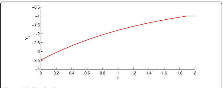
Finally, let us give a numerical simulation. Assume that the coefficients are all deter-ministic and time-invariant. Take c= ,d= ,T = ,δ =δ= ., B(t) =B(t) = ., Q= ,D(t) =D(t) = .,N(t) = ,α(t) = . In this case, it is easy to check thatZt=
for ≤t≤., andYtsolves the following ODE:
Yt= –.Yt+., ≤t≤; Y= –; Yt= , <t≤.,
which can be solved explicitly by subdividing [, ] backwardly to get
Yt= –, .≤t≤,
Yt= – – .(. –t), .≤t≤.,
.. .
The graph ofYtis shown in Figure . Then it is easy to check that +d
T
νtdt< , so we can takeC= . SincePt= –.Yt+.∈U, we can conclude that an adapted processuε· isε-optimal if it takes values inUand satisfies
E
Let us give an example ofε-optimal control for sufficiently smallε:
uεt = ⎧ ⎨ ⎩
–.Yt+.+ε/, ≤t≤.;
, . <t≤.
6 Conclusion
We study near-optimal controls for one kind of stochastic delay control problem with convex control domain. By the stochastic maximum principle and Ekeland’s variational principle, we establish necessary conditions for a control to be near-optimal. Sufficient conditions are also given, which show when an admissible control is indeed near-optimal. Two illustrative examples are given, for which some near-optimal controls in the explicit form are obtained. Future work includes the nonconvex control domain case and linear quadratic problems in terms of the Riccati equations.
Competing interests
The author declares that there is no competing interest regarding the publication of this paper.
Acknowledgements
The author would like to thank the editor and the reviewers for their valuable comments and suggestions that helped to improve this paper. This work is supported by the National Natural Science Foundation of China (11371228, 11471192), Natural Science Foundation of Shandong Province (ZR2015JL003, ZR2015JL021), Fostering Project of Dominant Discipline and Talent Team of Shandong Province Higher Education Institutions, Special Funds of Taishan Scholar Project
(tsqn20161041) and Project of Shandong Province Higher Educational Science and Technology Program (J15LI02).
Publisher’s Note
Springer Nature remains neutral with regard to jurisdictional claims in published maps and institutional affiliations.
Received: 18 November 2016 Accepted: 21 March 2017
References
1. Mohammed, SE: Stochastic Functional Differential Equations. Pitman, London (1984) 2. Mao, XR: Stochastic Differential Equations and Their Applications. Horwood, New York (1997)
3. Arriojas, M, Hu, Y, Mohammed, SE, Pap, G: A delayed Black and Scholes formula. Stoch. Anal. Appl.25(2), 471-492 (2007)
4. Elsanousi, I, Oksendal, B, Sulem, A: Some solvable stochastic control problems with delay. Stochastics71(1-2), 69-89 (2000)
5. Larrsen, B: Dynamic programming in stochastic control of systems with delay. Stochastics74(3), 651-673 (2002) 6. Oksendal, B, Sulem, A, Zhang, TS: Optimal control of stochastic delay equations and time-advanced backward
stochastic differential equations. Adv. Appl. Probab.43, 572-596 (2011)
7. Agram, N, Haadem, S, Oksendal, B, Proske, F: A maximum principle for infinite horizon delay equations. SIAM J. Math. Anal.45(4), 2499-2522 (2013)
8. Shen, Y, Meng, QX, Shi, P: Maximum principle for mean-field jump-diffusion stochastic delay differential equations and its application to finance. Automatica50(6), 1565-1579 (2014)
9. Peng, SG, Yang, Z: Anticipated backward stochastic differential equations. Ann. Probab.37(3), 877-902 (2009) 10. Chen, L, Wu, Z: Maximum principle for the stochastic optimal control problem with delay and application.
Automatica46(6), 1074-1080 (2010)
11. Yu, ZY: The stochastic maximum principle for optimal control problems of delay systems involving continuous and impulse controls. Automatica48(10), 2420-2432 (2012)
12. Huang, JH, Shi, JT: Maximum principle for optimal control of fully coupled forward-backward stochastic differential delayed equations. ESAIM Control Optim. Calc. Var.18(4), 1073-1096 (2012)
13. Du, H, Huang, JH, Qin, YL: A stochastic maximum principle for delayed mean-field stochastic differential equations and its applications. IEEE Trans. Autom. Control58(12), 3212-3217 (2013)
14. Zhou, XY: Stochastic near-optimal controls: necessary and sufficient conditions for near-optimality. SIAM J. Control Optim.36(3), 929-947 (1998)
15. Ekeland, I: On the variational principle. J. Math. Anal. Appl.47(2), 324-353 (1974)
16. Zhou, XY: Deterministic near-optimal controls. Part I: necessary and sufficient conditions for near optimality. J. Optim. Theory Appl.85(2), 473-488 (1995)
17. Zhou, XY: Deterministic near-optimal controls. Part II: dynamic programming and viscosity solution approach. Math. Oper. Res.21(3), 655-674 (1996)
19. Hafayed, M, Abbas, S, Veverka, P: On necessary and sufficient conditions for near-optimal singular stochastic controls. Optim. Lett.7(5), 949-966 (2013)
20. Hafayed, M, Abbas, S: Stochastic near-optimal singular controls for jump diffusions: necessary and sufficient conditions. J. Dyn. Control Syst.19(4), 503-517 (2013)
21. Hafayed, M, Abbas, S: On near-optimal mean-field stochastic singular controls: necessary and sufficient conditions for near-optimality. J. Optim. Theory Appl.160(3), 778-808 (2014)
22. Hafayed, M, Abba, A, Abbas, S: On mean-field stochastic maximum principle for near-optimal controls for Poisson jump diffusion with applications. Int. J. Dyn. Control2(3), 262-284 (2014)
23. Meng, QX, Shen, Y: A revisit to stochastic near-optimal controls: the critical case. Syst. Control Lett.82, 79-85 (2015) 24. Bahlali, K, Khelfallah, N, Mezerdi, B: Necessary and sufficient conditions for near-optimality in stochastic control of
FBSDEs. Syst. Control Lett.58, 857-864 (2009)
25. Huang, JH, Li, X, Wang, GC: Near-optimal control problems for linear forward-backward stochastic systems. Automatica46(2), 397-404 (2010)
26. Hafayed, M, Veverka, P, Abbas, S: On maximum principle of near-optimality for diffusions with jumps, with application to consumption-investment problem. Differ. Equ. Dyn. Syst.20(2), 111-125 (2012)
27. Hafayed, M, Veverka, P, Abbas, S: On near-optimal necessary and sufficient conditions for forward-backward stochastic systems with jumps, with applications to finance. Appl. Math.59(4), 407-440 (2014)
28. Zhang, LQ, Huang, JH, Li, X: Necessary condition for near optimal control of linear forward-backward stochastic differential equations. Int. J. Control88(8), 1594-1608 (2015)
29. Hafayed, M, Abba, A, Boukaf, S: On Zhou’s maximum principle for near-optimal control of mean-field