Performance of new BOC AW modulated signals for GNSS system

R E S E A R C H

Open Access

Performance of new BOC-AW-modulated signals

for GNSS system

Mustapha Flissi

, Khaled Rouabah

, Djamel Chikouche

, Abdehalim Mayouf

and Salim Atia

Abstract

In this paper, we propose efficient signal waveforms (WFs) with optimized spectrum for multipath (MP) mitigation and jamming reduction in global navigation satellite system. These WFs are based on the use of sine-phased binary offset carrier (BOC) with adjustable width (BOC-AW). They are generated by adjusting the width of the three-level WF {−1, 0, 1}. By exploiting the three-level BOC-AW subcarriers in sine-phasing signal model, we developed several forms of BOC-AW by means of superposition and width adjustment. The resulting power spectral densities and autocorrelation functions of the proposed WFs were calculated and introduced. Also calculated were the spectral separation coefficients (SSCs) and the Cramér-Rao lower bounds (CRLBs). The SSCs and CRLBs prove the efficiency of the proposed WFs in terms of interference separation. In addition, the simulation results show that the proposed WFs present better performances in MP mitigation compared to the WFs adopted by the Galileo and global positioning system modernization.

Keywords:GPS, Galileo, Multipath, BOC, MBOC, TMBOC, DLL, PN

Introduction

The binary offset carrier (BOC) modulation represents a serious candidate for global navigation satellite system (GNSS), especially for future global positioning system (GPS). Proposed by [1], the BOC modulation has several advantages compared to the traditional binary phase shift keying (BPSK), such as good spectral efficiency, high accuracy, enhanced multipath (MP) resolution [2], and better anti-jamming performances [3]. Other forms of modulation derived from the BOC concept are also used for new GPS and Galileo systems, such as quaternary phase shift keying modulation in L5 GPS signals [4], alternative BOC modulation in E5 Galileo signals [4], multiplexed BOC (MBOC) modulation with composite BOC (CBOC) implementation for Galileo, and time-multiplexed BOC (TMBOC) implementation for future GPS L1C [5]. Although these modulations are an import-ant innovation for GNSS systems, there are other modula-tions of great interest, such as binary coded symbol (BCS) modulation [6,7], composite binary coded symbols (CBCS) modulation [7], quadrature multiplexed BOC modulation

[8], minimum shift keying BOC modulation [9], multi-level subcarrier modulation specifically for three-multi-level or tertiary offset carrier (TOC) subcarrier modulation and five-level signals or 8-PSK subcarrier modulation [9,10], and m-PSK BOC modulation [11]. The 8-PSK signals achieve mostly better performances at lower bandwidth than comparable signal types. The effort to search for new signal waveforms (WFs) for navigation continues in order to propose a WF that has lower levels of interference with existing signals with an insurance of better performances in terms of MP mitigation and jamming reduction. In this paper, we propose efficient WFs for GNSS system which are labeled as sine-phased binary offset carrier with adjustable width (BOC-AW). These WFs are three-level (−1, 0, 1) and based on the sine-phased BOC concept with adjustable pulse width within each sub-carrier half cycle. A judicious choice of the pulse widths of the BOC-AW general mathematical model provides the general types of BOC and TOC WFs. The purpose of the proposed WFs is to eliminate components of the side lobes near the main lobe and at the same time increase the other side lobes of higher frequencies (far away from the main lobe) in order to get better per-formance in terms of MP and interference mitigation.

* Correspondence:[email protected]

1

LMSE Laboratory, Electronics Department, University of Bordj Bou Arréridj, Bordj Bou, Arréridj, Algeria

Full list of author information is available at the end of the article

BOC-AW(p,q,α(M)) modulation presents a sharper main peak due to the larger number of transitions of the sig-nal in the chip interval, which obviously corresponds to a greater slope of the discrimination function, allowing a reduction of MP effect. Also, BOC-AW modulations show better performances than BOC(p,p) and BOC(p,1) modulations for p > > 1 with regard to the receiving band. Moreover, both latter modulations have inconve-niences. In fact, BOC(p,q) WFs (q> > 1) need the use of several generator polynomials in contrast to the case whereq= 1, which uses only two generator polynomials. Also, it has been found that the tracking loop design for BOC(p,1) with p > > 1 may be more problematic than for BOC(1,1), especially with the conventional delay locked loop (DLL) algorithm with a narrow correlator. In effect, the BOC(p,1) ACFs withp> > 1, in contrast to that of BOC(1,1) modulation, produce several side peaks which complicate the DLL locking operation. The proposed WFs present also a better spectral separation and MP mitigation. Furthermore, they have better resist-ance against noise and jammer, and they can be used in conjunction with other MP mitigation techniques [12-15] for performance improvement.

This paper is organized as follows: firstly, we present the concept and the properties of BOC-AW-modulated WFs. Secondly, a general expression of the theoretical ACF and power spectral density (PSD) of BOC-AW WFs are presented. We present also the influence of pulse width adjustment on the structure of BOC-AW WF PSDs in comparison with their influence on that of BOC WF PSDs. Finally, the main performances of these proposed WFs are discussed and compared with the existing BOC and MBOC ones.

Proposed WFS and their properties

BOC is a square WF subcarrier modulation, where a signals(t) (the signal which is going to be modulated) is multiplied by a square WF subcarrier of frequency fs. Formally, the BOC-modulated signalsBOC(t) can be written as the product ofs(t) and sign(sin(2πfst)) [1,2].

For GNSS signals, the notation BOC(p,q) is used, where p and q are two indices satisfying the relation-ships

p¼fs½MHz=1:023 MHz½

and

q¼fc½MHz=1:023½MHz;

wherefcis the chip rate ofs(t).

The proposed BOC-AW subcarriers are three-level (−1, 0, 1) WFs with greater number of pulses in each

subcarrier half cycle compared to the BOC(1,1), TOC, and MBOC ones. The spreading signal in BOC-AW can be expressed as follows:

s tð Þ ¼ X

fornodd, whereTsis the half period of the subcarrier,n is the number of half period Ts during one code chip periodTc, Ck is the ki-th chip of the PRN code with fre-general model in Equation 3 for the different values of M and with judicious choice of α(M) are illustrated in Figure 1.

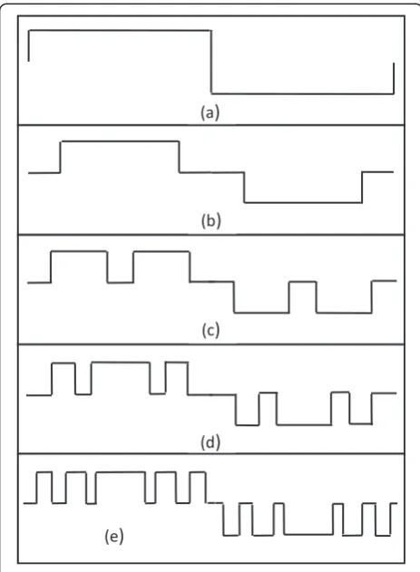
The expression of BOC(p,q) subcarrier used in Galileo and modernized GPS can be obtained easily from Equa-tion 3 (corresponding to our proposed WFs) withM =2 and α(2)=[α1=0, α2=1] (see Figure 1a). Similarly, the expression of TOC(p,q,α) [9,10] can also be determined from the same equation withM =2 andα(2)=[α1=α,α2=1] (see Figure 1b).

An example of three WFs is illustrated in Figure 1 (see Figure 1c,d,e). The WF of BOC-AW(p,q,α(4)) (Figure 1d) can be determined by the superposition of two WFs of BOC-AW(p,q,α(2)) (Figure 1c), one being defined by the

The BOC-AW WFS PSDs

Under the assumption that all the symbols are statisti-cally independent and equally probable, the PSDs of BOC-AW WFs with anti-polar binary code sequence can be established as follows:

G _ðp;q;αð ÞM_Þð Þ ¼f

In Equations 6 and 7, α′ indicates the active time where the signal adopts the values −1 and 1, and it is given as

forneven and

The sine-phased BOC(p,p) signal is characterized by fs= fc= p ×1.023 MHz andn= 2. Forneven, the differ-ence between the PSD of BOC-AW in Equation 6 and the PSD of BOC(p,p) in Equation 9 lies in the sine functions that contain theα(M)factors.

The aim is to use these functions to remove, by a judi-cious choice of the α(M) factors, some components of frequencies f = kfs in the PSD of BOC(p,p), more pre-cisely those corresponding to the maxima of secondary lobes (3fs, 5fs, 9fs…) that are nearer the principal lobes. Thus, we force the reduced power to be translated towards higher frequencies, which causes a positive impact on GNSS receiver performances.

To remove the frequency components kfs in the PSD of BOC-AW WFs, we solve the following equations:

XM

which forkodd can be further simplified to

XM

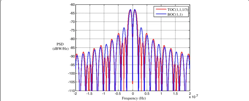
For this case, we find the TOC signal (Figure 1b) and a system of equations given by

cos π

This system admits only one solution, which means that we can delete only one frequency component. Figure 2 shows that the PSD of TOC(1,1,α1= 1/3) presents a simi-lar spectral density to that of BOC(1,1) but introduces additional zeros at 3fs, 9fs, 15fs, 21fs….

Case 2: M = 2 and 0 <α1<α2< 1

This case permits determination and elimination of the terms of both frequencies k1fs and k2fs by solving the following system of equations:

X2

The solution shows that the exact values of α1and α2 are obtained whenk1= 3andk2=7.

introduces additional zeros at 3fsand 7fsand strengthens the other components of the PSD.

Case 3: M = 4 and 0 <α1<α2<α3<α4= 1

This case corresponds to BOC-AW(1,1,α(4)) WF

(Figure 1d). This WF is defined by four factors, α1, α2, α3, andα4= 1, whose judicious choice eliminates the fre-quency components 3fs, 5fs, and 7fs in the BOC(p,p) PSD.

In order to delete three frequency components that correspond to k1, k2, and k3, the three values α1, α2, and α3must be found by solving the following system

of equations:

Figure 4 shows the BOC(1,1) and the resulting BOC-AW(1,1,α(4)) PSDs. Note that the PSD of BOC-AW

Figure 3Normalized PSDs of BOC-AW(1,1,α(2)) and BOC(1,1).

-2 -1.5 -1 -0.5 0 0.5 1 1.5 2

(1,1,α(4)) compared to that of BOC(1,1) introduces additional zeros at 3fs, 5fs, and 7fsand increases power at higher frequencies.

Case 4: M = 6 and 0 <α1<α2<α3<α4<α5<α6= 1

This last case represents the BOC-AW(1,1,α(6)) WF (Figure 1e) with six factors, α(6). BOC-AW(1,1,α(6)) is used with a judicious choice of factors, α(6), to delete five frequency components (3fs, 5fs, 7fs, 9fs, and 11fs) in BOC(1,1) PSD.

To do this, we must solve the system of equations given as

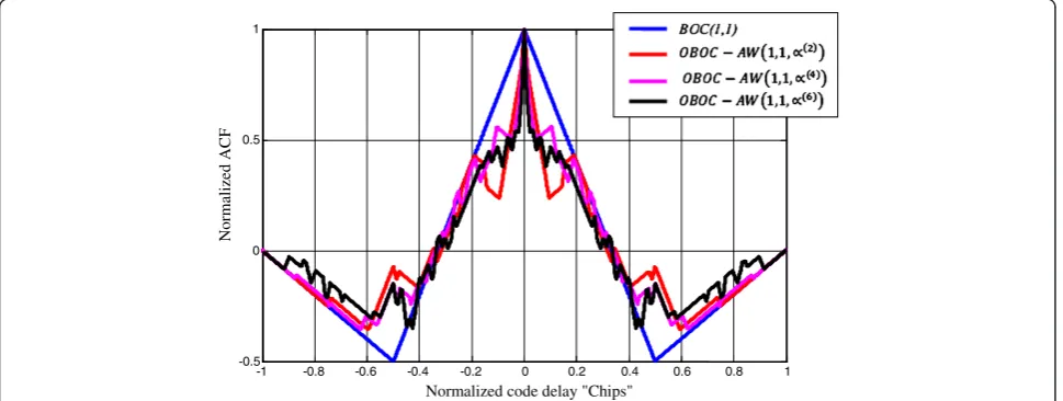
Figure 5 shows the BOC(1,1) and the resulting BOC-AW(1,1,α(6)) PSDs. Note that the PSD of BOC-AW (1,1,α(6)) compared to that of BOC(1,1) introduces additional zeros at 3fs, 5fs, 7fs, 9fs, and 11fs and in-creases power at higher frequencies. Figure 6 shows the ACFs of different BOC-AW versions and BOC modulations.

It is clear that the ACFs of BOC-AW yield sharper peaks with respect to that of BOC(1,1). This causes an improvement of the code tracking performance, as we are going to see in the last part of this paper.

Noise-induced code tracking error

The Cramér-Rao lower bound (CRLB) is the lower bound of the root mean square error (RMSE) for any estimate

of a nonrandom parameter. The CRLB can be expressed as [9,15]

where BLrefers to the loop bandwidth of the code track-ing loop,C/N0is the carrier-to-noise ratio, andR″ss(τ) and Gs(f) are respectively the ACF and the PSD of the signal. In order to understand how the code tracking noise be-haves for the set of modulations considered in this paper, we present in Figures 7, 8, 9 the CRLB using respectively 5, 12, and 24 MHz receiving bandwidths (double-sided) andBL= 0.2 Hz.

Figure 7 shows that the proposed BOC-AW modula-tions, with 5 MHz bandwidth, provide a much better code tracking accuracy than TMBOC(6,1,4/33), CBOC (6,1,1/11) pilot, CBCS([1,−1,1,−1,1,−1,1,−1,1,1],1,20%), and BOC(1,1) modulations. As we can recognize in Figure 8, for 12 MHz receiving bandwidth, the best per-formance is given by CBCS([1,−1,1,−1,1,−1,1,−1,1,1],1,20%), followed by BOC-AW(1,1,α(2)), whereas all other modula-tions clearly outperform BOC-AW(1,1,α(4)) and BOC-AW (1,1,α(6)).

Figure 9 shows that the proposed modulations BOC-AW(1,1,α(2)) and BOC-AW(1,1,α(4)) with 24 MHz bandwidth provide the best code tracking accuracy. However, all other modulations clearly outperform BOC-AW(1,1,α(6)).

RMS bandwidth and cumulative PSDs

The root mean square bandwidth (RMSB) can also be seen as another way of interpreting the CRLB or as the

-2 -1.5 -1 -0.5 0 0.5 1 1.5 2

Gabor bandwidth of a signal [9]. The RMSB can be expressed as [1,9]

βrmsð Þ¼Br

ffiffiffiffiffiffiffiffiffiffiffiffiffiffiffiffiffiffiffiffiffiffiffiffiffiffiffiffiffiffiffiffiffiffiffiffiffiffiffiffiffiffiffiffiffiffiffiffiffiffiffiffiffiffiffiffiffiffiffiffiffiffi

∫Br=2 −Br=2 f

2―_G sð Þf df q

ð20Þ

where Gs ð Þf is the normalized PSD over receiver front-end bandwidthBr.

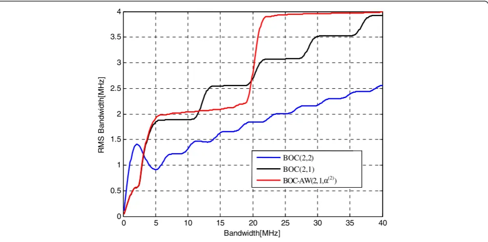
Figures 10 and 11 show respectively the RMSB and the cumulative normalized PSDs of different modula-tions. As we can notice, for the 24 MHz receiving bandwidth, the RMSBs of BOC-AW(1,1,α(2)) and

BOC-AW(1,1,α(4)) are much greater than that of any other modulation, while the RMSB of BOC-AW(2,α(6)) is the smallest. Ninety percent of the BOC-AW(1,1,α(2)) power is reached within a frequency band less than 12 MHz. This is approximately the same case for CBCS ([1,−1,1,−1,1,−1,1,−1,1,1],1,20%) modulation. Never-theless, 90% of both TMBOC(6,1,4/33) and CBOC (6,1,1/11) powers is situated in a frequency band greater than 12 MHz. The bandwidths including 90% of the BOC-AW(1,1,α(4)) and BOC-AW(1,1,α(6)) pow-ers are much wider than those including that of BOC

-1.5 -1 -0.5 0 0.5 1 1.5

-0.5 0 0.5 1

Normalized code delay “chips” Normalized

ACF

BOC-AW (1,1,(6) ) BOC-AW (1,1,(4)

) BOC-AW (1,1,(2)

) BOC(1,1)

Figure 6Normalized ACFs of BOC-AW(1,1,α(2)_{), BOC-AW(1,1,α}(4)_{), BOC-AW(1,1,α}(6)_{), and BOC(1,1).}

20 25 30 35 40 45 50

0 1 2 3 4 5 6 7

C/N0[dB-Hz]

C

ode n

oi

s

e(

m

)

BOC(1, 1)

CBCS([1,-1,1,-1,1,-1,1,-1,1,1],1, 20%)

BOC-AW(1,1, (2)₎

CBOC(1, 6, 1/11) TMBOC(1, 6, 4/33)

BOC-AW(1,1, (4)₎

BOC-AW(1,1, (6)₎

Figure 7CRLB of TOC(1,1,1/3), BOC(1,1), CBCS([1,−1,1,−1,1,−1,1,−1,1,1],1,20%), BOC-AW(1,1,α(2)_{), CBOC(6,1,1/11), TMBOC(6,1,4/33),}

(1,1), CBCS([1,−1,1,−1,1,−1,1,−1,1,1],1,20%), TMBOC (6,1,4/33), and CBOC(6,1,1/11) powers.

Figure 12 shows the RMSBs of BOC(2,2), BOC(2,1), and BOC-AW(2,1,α(2)) modulations withp= 2 andq= 1. As we can recognize, for 5, 12, and 24 MHz receiving bandwidths, the RMSB of BOC-AW(2,1,α(2)) modulation is much greater than those of BOC(2,2) and BOC(2,1) modulations.

Spectral separation coefficient

SSC is a very important tool to design a new signal with better relevance for coexistence with GNSS signals in the same frequency band. In fact, the SSC concept provides a measure of the noise power output from a receiver when certain signals, with given spectra, are in-cident at its input. This shows that the fundamental measure is a cross PSD [10,16].

20 25 30 35 40 45 50

0 1 2 3 4 5 6

C/N0[dB-Hz]

C

ode n

oi

s

e(

m

)

BOC(1, 1)

CBCS([1,-1,1,-1,1,-1,1,-1,1,1],1, 20%)

BOC-AW(1,1, (2))

CBOC(1, 6, 1/11) TMBOC(1, 6, 4/33)

BOC-AW(1,1, (4))

BOC-AW(1,1, (6))

Figure 8CRLB of TOC(1,1,1/3), BOC(1,1), CBCS([1,−1,1,−1,1,−1,1,−1,1,1],1,20%), BOC-AW(2,α(2)_{), CBOC(6,1,1/11), TMBOC(6,1,4/33),}

BOC-AW(1,1,α(4)_{), and BOC-AW(1,1,α}(6)_{) to 12 MHz receiving bandwidth.}

20 25 30 35 40 45 50

0 0.5 1 1.5 2 2.5 3 3.5 4 4.5 5

C/N0[dB-Hz]

C

ode n

o

is

e(

m

)

BOC(1, 1)

CBCS([1,-1,1,-1,1,-1,1,-1,1,1],1, 20%) BOC-AW(1,1, (2)₎

CBOC(1, 6, 1/11) TMBOC(1, 6, 4/33) BOC-AW(1,1, (4)₎

BOC-AW(1,1, (6))

Figure 9CRLB of TOC(1,1,1/3), BOC(1,1), CBCS([1,−1,1,−1,1,−1,1,−1,1,1],1,20%), BOC-AW(1,1,α(2)_{), CBOC(6,1,1/11), TMBOC(6,1,4/33),}

The SSC between desired signal and interfering signal can be expressed as [1]

kis¼ Z

−Br=2

Br=2 _Gsð Þ_{f Gi}ð Þ_{f df}

ð21Þ

where Br is the receiver front-end filter bandwidth, and Gs(f) and Gi(f) are respectively the normalized PSD of

the desired signal and interfering signal. In Table 1, sev-eral SSC results are given for the case of infinite trans-mission bandwidth and a 24 MHz receiver bandwidth.

As we can recognize from this table, the BOC-AW (1,1,α(6)) WF presents better spectral separation with the GNSS WFs E1/L1. For example, the SSC for BOC-AW (1,1,α(6)) with GPS coarse acquisition (C/A) code is 0.5 dB higher than that for BOC(1,1) with the same code. BOC-AW(1,1,α(2)) and BOC-AW(1,1,α(4)) WFs present

0 5 10 15 20 25 30 35 40

0 1 2 3 4 5 6

Bandwidth[MHz]

R

M

S Ba

n

d

w

id

th

[M

H

z

]

BOC(1,1)

CBCS([1,-1,1,-1,1,-1,1,-1,1,1],1,20%)

BOC-AW(1,1, (2)₎

CBOC(1,6,1/11) TMBOC(1,6,4/33)

BOC-AW(1,1, (4)₎

BOC-AW(1,1, (6))

Figure 10RMSEs of the different WFs.

0 5 10 15 20 25 30 35 40

0 0.1 0.2 0.3 0.4 0.5 0.6 0.7 0.8 0.9 1

Bandwidth[MHz]

F

rac

ti

ona

l P

o

w

er

Lo

s

s

BOC(1,1)

CBCS([1,-1,1,-1,1,-1,1,-1,1,1],1,20%) BOC-AW(1,1, (2))

CBOC(1,6,1/11) TMBOC(1,6,4/33) BOC-AW(1,1, (4)) BOC-AW(1,1, (6)₎

less spectral overlapping with GPS P(Y), GPS C/A, GPS L1C, and Galileo E1 open service (OS) WFs. Also, the SSCs for BOC-AW(1,1,α(2)) and BOC-AW(1,1,α(4)) with GPS C/A code are respectively 0.48 and 0.27 dB higher than that for BOC(1,1) with the same code. However, the SSCs for BOC(1,1) WF with GPS M code and with Galileo E1 public regulated service (PRS) are respectively higher than those for BOC-AW(1,1,α(2)) and BOC-AW (1,1,α(4)) with GPS M code and with Galileo E1 PRS.

Real implementation of the proposed waveforms

In reality, difficulty exists when directly applying the original WFs in the GNSS system. It is mainly due to the use of three-level WFs, including a zero level. In fact, this may lead to large power fluctuations of the radio frequency (RF) signal, which is a highly undesir-able feature and represents a limitation in the practi-cality of our method. To overcome this problem, the proposed WFs were time multiplexed with BOC(Mp,p) WFs. As a result, the zero transitions in BOC-AW WFs are occupied by a BOC(Mp,p) WF. These optimized

BOC-AW (OBOC-AW) WFs are a constant envelope and bring another important quantity of energy at high frequencies that is added to that brought by the pro-posed original ones. This combination can be given as follows:

SOBOCAWð Þ ¼t SBOCAWð Þt

if jSBOCAWð Þt j ¼1 SBOCðMp;pÞð Þt otherwise :

ð22Þ

OBOC-AW(p,p,α(2)), OBOC-AW(p,p,α(4)), and OBOC-AW(p,p,α(6)) are shown respectively at the top, middle, and bottom of Figure 13.

The ACFs of both the BOC(1,1) and OBOC-AW (p,p,α(M)) WFs are illustrated in Figure 14. As illustrated in Figure 14, by performing this combination, a much sharper correlation peak can be achieved in practice. In addition, the resulting ACFs present side peaks with smaller levels compared to the BOC(1,1) ones. This will cause a small perturbation at the DLL in terms of ambi-guity, and thus it will present the best performances in

0 5 10 15 20 25 30 35 40

0 0.5 1 1.5 2 2.5 3 3.5 4

Bandwidth[MHz]

RM

S

B

a

n

d

wi

d

th

[M

H

z

]

BOC(2,2) BOC(2,1) BOC-AW(2, 1, (2)₎

Figure 12RMSEs of BOC(2,1), BOC(2,2), and BOC-AW(2,1,α(2)_).

Table 1 SSCs (dB) between BOC(1,1), TOC(1,1,1/3), BOC-AW, and GNSS E1/L1 signals

Signal GPS P (Y) GPS C/A GPS M Galileo E1 PRS GPS L1C

code code code BOCc(15,2.5) Galileo E1 OS

BPSK(10) BPSK(1) BOC(10,5) MBOC(6,1,1/11)

BOC(1,1) −69.1191 −73.5871 −81.8083 −103.3613 −62.5287

TOC(1,1,1/3) −69.3055 −73.8123 −81.7546 −103.1296 −62.9200 BOC-AW(1,1,_α(2)₎

−69.5970 ₋74.2102 ₋81.7456 ₋97.9512 ₋63.3452 BOC-AW(1,1,α(4)_{) −69.3835 −73.7856 −80.4395 −97.3670 −62.8448}

positioning the receiver, as we are going to see in the last part of this paper.

Simulation results

Simulations were conducted to test the performances of the proposed WFs. For this reason, three situations were presented.

In the first situation, 11 schemes have been simu-lated. The first five were based respectively on BOC (1,1), CBOC, TMBOC, TOC, and CBCS WFs. The last six schemes were based on our proposed WFs with BOC-AW configuration (BOC-AW(1,1,α(2)), BOC-AW (1,1,α(4)), and BOC-AW(1,1,α(6))) and with OBOC-AW configuration (OBOC-AW(1,1,α(2)), OBOC-AW(1,1,α(4)),

and OBOC-AW(1,1,α(6))). In this first situation, we con-sider MP channel constructed with a line-of-sight (LOS) signal and a single reflected signal. Three different values of the pre-correlation bandwidth were chosen (5, 12, and 24 MHz) to estimate the MP error envelopes of all 11 schemes. The MP signal has an amplitude of 0.5 and is varied in delay from 0 to 450 m with respect to the LOS delay. The MP error envelopes, which are calculated at the maximum points (when the MP signal is at 0°‘in phase’or 180° ‘out of phase’with respect to the LOS) are used to calculate the running average errors. The principle of this consists in calculating the absolute envelope values and their cumulative sum with the aim of computing the aver-age running errors. The norm used herein is that used in 0 0.1 0.2 0.3 0.4 0.5 0.6 0.7 0.8 0.9 1

-1 0 1

0 0.1 0.2 0.3 0.4 0.5 0.6 0.7 0.8 0.9 1 -1

0 1

0 0.1 0.2 0.3 0.4 0.5 0.6 0.7 0.8 0.9 1 -1

0 1

Time index in "Chips" _Original

Optimized

Figure 13Original and optimized WFs.

-1 -0.8 -0.6 -0.4 -0.2 0 0.2 0.4 0.6 0.8 1 -0.5

0 0.5 1

Normalized code delay "Chips"

Nor

m

al

ize

d

ACF

0 50 100 150 200 250 300 350 400 0

1 2 3 4 5 6

Relative MP delays in "Meters"

Running Av

erag

e e

rro

r in "Met

ers

"

Figure 15Running average errors of the different WFs with a pre-correlation bandwidth of 5 MHz.

0 50 100 150 200 250 300 350 400

0 1 2 3 4 5 6

Relative MP delays in "Meters"

Running Av

erag

e e

rro

r in "Meters

"

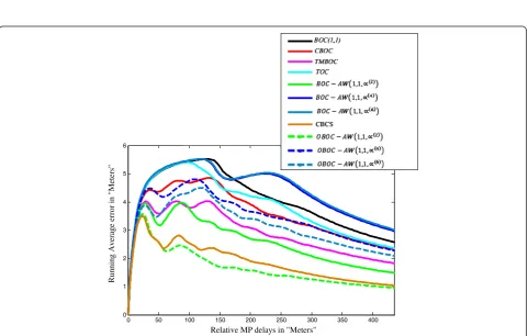
reference [17]. The results, for the different band-limited ACFs, are shown in Figures 15, 16, 17.

As exposed in Figure 15, which corresponds to 5 MHz pre-correlation bandwidth, the running average errors of the scheme based on our proposed WFs decrease toward small values from a delay which is greater than approxi-mately 150 m with respect to the LOS. BOC-AW(1,1,α(2)), BOC-AW(1,1,α(4)), and BOC-AW(1,1,α(6)) show the best performances for all MP delays greater than 125 m except for MP delays between 170 and 250 m where the best performances are given by the CBCS scheme. OBOC-AW (1,1,α(2)), OBOC-AW(1,1,α(4)), OBOC-AW(1,1,α(6)), TOC, CBOC, BOC(1,1), and TMBOC have similar performances for MP delays greater than approximately 200 m and present the worst schemes for MP delays in that range. However, for MP delays between 150 and 200 m, it is the OBOC-AW(1,1,α(2)) which represents the worst perfor-mances followed by OBOC-AW(1,1,α(4)). This can be explained by the fact that the DSPs of our proposed BOC-AW WFs present the largest principal lobes. Also, the performance degradation of the OBOC-AW WFs is due to the fact that their enhanced frequency components lie outside the 5 MHz pre-correlation bandwidth.

In Figure 16 where the pre-correlation bandwidth is chosen equal to 12 MHz, both BOC-AW(1,1,α(4)) and BOC-AW(1,1,α(6)) WFs present the worst performances while BOC-AW(1,1,α(2)) performs better than all the

modulation schemes except for OBOC-AW(1,1,α(2)) and CBCS. OBOC-AW(1,1,α(2)) and CBCS show almost the same performances for delay values below 60 m, while OBOC-AW(1,1,α(2)) performs better for delay values greater than 60 m. Finally, it should be noted that OBOC-AW(1,1,α(4)) and OBOC-AW(1,1,α(6)) WF per-formances are between those of CBOC and TMBOC.

In Figure 17, which corresponds to a 24 MHz pre-correlation bandwidth, the OBOC-AW(1,1,α(4)) WFs present the best performances for all the band of varia-tions of the MP delay with a maximum error of approxi-mately 1.8 m. The latter is followed by OBOC-AW (1,1,α(6)) which gives the best performances than all the remaining schemes for delays greater than approximately 30 m. For delays greater than approximately 60 m, OBOC-AW(1,1,α(2)) shows better performances than all the remaining WFs. Besides, BOC-AW(1,1,α(2)) and BOC-AW(1,1,α(4)) performances are close to those of CBCS, TMBOC, and CBOC and better than those of TOC and BOC(1,1) WFs. BOC-AW(1,1,α(6)) presents the worst case. In addition to the MP perturbation, another limita-tion exists, which is the presence of noise. To test the robustness of our proposed WFsvis-à-visthe noise, we present the second situation. For this, all the previous schemes are firstly simulated. Then a comparison is ac-complished between their code tracking RMSEs for three different values of the pre-correlation bandwidth

0 50 100 150 200 250 300 350 400

0 1 2 3 4 5 6

Relative MP delays in "Meters"

Running Av

erag

e e

rro

r i

n

"Met

ers

"

(5, 12, and 24 MHz). The results are shown respect-ively in Figures 18, 19, 20.

The RMSEs are represented versus signal-to-noise ratio (SNR) which varies from−35 to−20 dB. The SNR is defined as the (C/N0) divided by the RF signal bandwidth.

In Figure 18, corresponding to 5 MHz pre-correlation bandwidth, the RMSEs of all our WFs approach those of all the other WFs. In Figure 19, we observe that for a 12 MHz pre-correlation bandwidth, the OBOC-AW(1,1,α(2)) together with the CBCS WF shows the best perfor-mances regardless of the SNR value. For the 24 MHz

-35 -30 -25 -20

0.5 1 1.5 2 2.5 3 3.5 4

SNR in "dB"

RMSE in

"M

ete

rs

"

Figure 18RMSEs of the different WFs with pre-correlation bandwidth of 5 MHz.

-35 -30 -25 -20

0 0.5 1 1.5 2 2.5 3 3.5 4

SNR in "dB"

RMSE in

"M

ete

rs

"

pre-correlation bandwidth, as shown in Figure 20, OBOC-AW(1,1,α(2)) and OBOC-AW(1,1,α(4)) present the smallest RMSEs in comparison with the other WFs, which shows their robustness concerning the noise and the efficiency of our proposed waveforms. OBOC-AW (1,1,α(4)) presents the same RMSE with that of CBCS.

The final situation is realized to compare the RMSEs of our OBOC-AW WFs with those of BOC(15,2.5) WF which has a high modulation order and lies in the same frequency band. The simulation results for 5, 12, and 24 MHz are given respectively in Figures 21, 22 and 23. As shown in these figures, our WFs present the best performances vis-à-vis the noise. This result is valid for all pre-correlation bandwidth values.

Conclusions

In this paper, efficient WFs for MP mitigation and inter-ference reduction in GNSS system are proposed. For this purpose, both BOC-AW and OBOC-AW WF con-figurations were presented and compared to the existing BOC WFs. BOC-AW WFs, although they present better performances than BOC ones, might suffer from power fluctuations caused by zero level. However, this problem is completely resolved by using OBOC-AW WFs. Be-sides, due to their ACF forms, OBOC-AW WFs are shown to have superior performance improvement in terms of MP error and delay variation band reduction. Among these, the OBOC-AW(1,1,α(2)) WF is found to be undoubtedly the best. In addition, the proposed

-35 -30 -25 -20

0 0.5 1 1.5 2 2.5 3 3.5

SNR in "dB"

RMSE in

"M

ete

rs

"

Figure 20RMSEs of the different WFs with pre-correlation bandwidth of 24 MHz.

-35 -30 -25 -20

0 1 2 3 4 5 6 7 8

RMSE in

"M

ete

rs

"

SNR in "dB"

BOC(15,2.5) OBOC-AW(p,p,α(2)

)

OBOC-AW(p,p,α(6)) OBOC-AW(p,p,α(4)

)

WFs present better resistance to noise and jamming due to their DSP distributions which present important quantities of power at high frequencies. Moreover, the scheme with these WFs works for both short/long and weak/strong MP.

Appendix

Calculation of BOC-AW PSD

Accepting the assumption given above, the PSD of the BOC-AW signal is given by

G _ðp;q;αð ÞM_Þð Þ ¼f

SBOCAW _ðp;q;αð ÞM_Þð Þf

2

Tc ð

23Þ

whereSBOC-AW(p,q,α(M))(f) is the Fourier transform of subcarrier WFsBOC-AW(p,q,α(M))(t).

In Equation 3, the Fourier transform of X 1

i¼0

pl;iðt−mTsÞ is given as

e−j2πfmTs

πfejπfTs ½sinðπf 1ð −α2l−1ÞTsÞ−sinðπf 1ð −α2lÞTsÞ: ð24Þ

Thus, the Fourier transform of the spreading symbol sBOC-AW(p,q,(αM))(t) is given as follows:

SBOCAW _ðp;q;αð ÞM_Þð Þ ¼f 1 πf ejπf Ts

XM=2

l¼1

½sinðπfð1−α2l−1ÞTsÞ þ

−sinðπfð1−α2lÞTsÞ

Xn−1

m¼0

−1

ð Þm

e−j2πfmTs:

ð25Þ

-35 -30 -25 -20

0 1 2 3 4 5 6

SNR in "dB"

RMSE in

"M

ete

rs

"

BOC(15,2.5) OBOC-AW(p,p,α(2)₎

OBOC-AW(p,p,α(6)₎

OBOC-AW(p,p,α(4))

Figure 22Comparison of RMSEs of our proposed WFs and BOC(15,2.5) with pre-correlation bandwidth of 12 MHz.

-35 -30 -25 -20

0 0.2 0.4 0.6 0.8 1 1.2 1.4

SNR in "dB"

RMSE in

"M

ete

rs

"

BOC(15,2.5) OBOC-AW(p,p,α(2))

OBOC-AW(p,p,α(6)₎

OBOC-AW(p,p,α(4))

The summation

Substitution of Equation 26 into Equation 25 yields

SBOCAW _ðn;αð ÞM_Þð Þ ¼f je

Substitution of Equation 28 into Equation 25, yields

sBOCAW _ðp;q;αð ÞM_Þð Þ ¼f e

Finally, the PSD for the BOC-AW signal is given as

G _ðp;q;αð ÞM_Þð Þ ¼f

for n odd, whereα′ indicates the active time where the signal adopts the values {−1, 1}, and it is given as

ACF:autocorrelation function; BCS: binary coded symbol; BOC: binary offset carrier; BOC-AW: binary offset carrier with adjustable width; BPSK: binary phase shift keying; C/A: coarse acquisition; CBCS: composite binary coded symbols; CBOC: composite BOC; CRLB: Cramér-Rao lower bound; DLL: delay locked loop; GNSS: global navigation satellite systems; GPS: global positioning system; LOS: line of sight; MBOC: multiplexed BOC; MP: multipath; OBOC-AW: optimized BOC-AW; PRS: public regulated service; PSD: power spectral density; RMSEs: root mean square errors; SNR: signal-to-noise ratio; SSC: spectral separation coefficient; TOC: tertiary offset carrier; WF: waveform.

Competing interests

The authors declare that they have no competing interests.

Acknowledgments

The authors would like to thank Prof. Abderrahmane Bendaas, rector of the University of Bordj Bou Arréridj, for his moral support.

Author details

1

LMSE Laboratory, Electronics Department, University of Bordj Bou Arréridj, Bordj Bou, Arréridj, Algeria.2_{LIS Laboratory, Electronics Department,}

University of M'sila, M'sila, Algeria.3DMMER Laboratory, Electronics Department, Ziane Achour University of Djelfa, Djelfa, Algeria.

Received: 16 May 2012 Accepted: 8 April 2013 Published: 9 May 2013

References

1. JW Betz, The offset carrier modulation for GPS modernization, inProceedings

of ION Technical Meeting(San Diego). 25–27 January 1999, pp. 639–648

2. JW Betz, Binary offset carrier modulations for radionavigation. J The Institute of Navigation48, 227–246 (2001)

3. J Chen, YG Zhang, GB Liang, F Li, The anti-jamming performance of GNSS BOC signals in certain jamming environments, inProceeding of ISAPE 2008: The 8th International Symposium on Antennas, Propagation and EM Theory,

vol. 1–3(Kunming). 2–5 November 2008

4. Galileo Open Service, Signal in space interface control document, European Space Agency/Galileo Joint Undertaking, Draft GAL OS SIS ICD/D.0. (2006) 5. GW Hein, JA Avila-Rodriguez, S Wallner, AR Pratt, MBOC: the new optimized

spreading modulation recommended for Galileo L1 OS and GPS L1C, in

Proceedings of the IEEE/ION Position, Location, and Navigation Symposium

(San Diego), p. 25–27 April 2006, pp. 883–892

6. CJ Hegarty, JW Betz, A Saidi, Binary coded symbol modulations for GNSS, in

Proceedings of the 60th Annual Meeting of the Institute of Navigation, ION-NTM(Dayton). 7–9 June 2004

7. GW Hein, JA Avila-Rodriguez, L Ries, L Lestarquit, J-L Issler, J Godet, AR Pratt, Galileo Signal Task Force of the European Commission, A candidate for the Galileo L1 OS optimized signal, inProceedings of the 18th International Technical Meeting of the Satellite Division of the Institute of Navigation

(ION-GNSS)(Long Beach). 13–16 September 2005

8. Z Yao, M Lu, ZM Feng, Quadrature multiplexed BOC modulation for interoperable GNSS signals. Electron Lett46, 1234–1236

9. JA Avila-Rodriguez,On generalized signal WFs for satellite navigation, PhD

Thesis(University FAF Munich, Neubiberg, Germany, 2008)

10. AR Pratt, JIR Owen, BOC modulation WFs, inION Proceedings, GPS 2003

Conference(Portland). 9–12 September 2003

11. AR Pratt, JIR Owen, Performance of GPS/Galileo receivers using m-PSK BOC signals, inProceedings of the 2004 National Technical Meeting of the Institute

of Navigation(San Diego). 26–28 January 2003

12. K Rouabah, D Chikouche, F Bouttout, R Harba, and P Ravier,“GPS/galileo multipath mitigation using the first side peak of double delta correlator”, Wireless Personal Communications,60, 2, pp. 321–333, (2010). 13. K Rouabah, D Chikouche, GPS/Galileo multipath detection and mitigation

using closed-form solutions. Math Probl Eng, (2009). doi:10.1155/2009/ 106870

14. M Sahmoudi, MG Amin, Fast iterative maximum-likelihood algorithm (FIMLA) for multipath mitigation in the next generation of GNSS receivers. IEEE Trans Wirel Commun7, 4362–4374 (2008)

Technical Meeting of the Institute of Navigation, ION-GNSS 2006(Fort Worth Convention Center, Fort Worth). 26–29 September 2006

16. JW Betz, Effect of partial-band interference on receiver estimation of C/N0: theory, inProceedings of the National Technical Meeting of the Institute of

Navigation ION-NTM 2001(Long Beach). 22–24 January 2001, pp. 16–27

17. M Irsigler, JA Avila-Rodriguez, GW Hein, Criteria for GNSS multipath performance assessment, inProceedings of the International Technical

Meeting of the Institute of Navigation (ION-GNSS 2005)(Long Beach).

13–16 September 2005

doi:10.1186/1687-1499-2013-124

Cite this article as:Flissiet al.:Performance of new BOC-AW-modulated signals for GNSS system.EURASIP Journal on Wireless Communications and Networking20132013:124.

Submit your manuscript to a

journal and benefi t from:

7 Convenient online submission 7 Rigorous peer review

7 Immediate publication on acceptance 7 Open access: articles freely available online 7 High visibility within the fi eld

7 Retaining the copyright to your article