R E S E A R C H
Open Access
Cascaded orthogonal space–time block codes
for wireless multi-hop relay networks
Rahul Vaze
1*and Robert W Heath Jr.
2Abstract
Distributed space–time block coding is a diversity technique to mitigate the effects of fading in multi-hop wireless networks, where multiple relay stages are used by a source to communicate with its destination. This article proposes a new distributed space–time block code called the cascaded orthogonal space–time block code (COSTBC) for the case where the source and destination are equipped with multiple antennas and each relay stage has one or more multiple antenna relays. Each relay stage is assumed to have receive channel state information (CSI) for all the
channels from the source and all relays from previous stages to itself, while the destination is assumed to have receive CSI for all the channels. To construct the COSTBC, multiple orthogonal space–time block codes (OSTBCs) are used in cascade by the source and each relay stages. In the COSTBC, each relay stage separates the constellation symbols of the OSTBC sent by the preceding relay stage using its CSI, and then transmits another OSTBC to the next relay stage. COSTBCs are shown to achieve the maximum diversity gain in a multi-hop wireless network with linear decoding complexity thanks to the connection to OSTBCs. Several explicit constructions of COSTBCs are also provided, and their performance is simulated in different relay configurations.
1 Introduction
Distributed space–time block coding (DSTBC) is a technique to improve reliability in relay-assisted communication, where one or more relays help the source to communicate with its destination. Relay-assisted com-munication is likely to occur in large wireless networks, such as ad-hoc or sensor network, where the destination is possibly out of the source’s communication range. Relay-assisted communication is also used in a cellular wireless networks to improve the performance of cell edge users, and has been incorporated in modern wireless standards such as IEEE 802.16j, and 3GPP LTE Advanced. In DSTBCs, relay antennas are used together with the source antennas in a distributed manner to transmit a space–time block code (STBC) [1] to the destination. By introducing redundancy in space and time, DSTBCs increase the reliability of the communication by increas-ing the diversity gain, defined as the negative of the expo-nent of the signal-to-noise ratio (SNR) in the pairwise error probability expression at high SNR [1].
*Correspondence: [email protected]
1School of Technology and Computer Science, Tata Institute of Fundamental Research, Mumbai 400005, India
Full list of author information is available at the end of the article
In prior work, maximum diversity gain achieving DSTBC constructions have been proposed for the two-hop network [2-21], and for the multi-two-hop network [22-24]. Even though these DSTBC constructions [2-24] achieve the maximum diversity gain, the decoding com-plexity of most of them, except [14-21], is very high, thereby limiting their use in practical deployment. Con-struction of DSTBCs with low decoding complexity is practically important as highlighted by the fact that the Alamouti code is the most practically used code not only because it achieves the maximum diversity gain, but also because it requires minimum decoding complexity. Moreover, the DSTBC constructions with low decoding complexity [14-21] are limited to two-hop network with single antenna equipped source, destination, and the relay nodes.
In this article, we design maximum diversity gain achieving DSTBCs with low-decoding complexity for a multi-hop wireless network where the source, the desti-nation, and the relay nodes are equipped with multiple antennas. In the proposed DSTBC, called the cascaded orthogonal space–time block code (COSTBC), an orthog-onal space-time code (OSTBC) [25] is used by the source, and subsequently by each relay stage to communicate with its adjacent relay stage. OSTBCs are considered because
of their single symbol decodable property [25,26], i.e., with the maximum likelihood decoding each constellation symbol of the OSTBC can be decoded independently of other constellation symbols. We assume that each relay has receive channel state information (CSI) for all the channels from the source to itself, while the destination is assumed to have receive CSI for all the channels. With COSTBCs, in the first time slot, the source transmits an OSTBC to the first relay stage. Using the orthogonal-ity property of the OSTBC and the available CSI, each relay of the first relay stage separates the different OSTBC constellation symbols from the received signal, and trans-mits a codeword vector in the next time slot, such that the matrix obtained by stacking all the codeword vectors transmitted by the different relays of the first relay stage is an OSTBC. These operations are repeated by subse-quent relay stages. With COSTBCs, no signal is decoded at any of the relays, therefore COSTBC construction with single antenna relays is equivalent to COSTBC construc-tion with multiple antenna relays. Thus, without loss of generality, in this article, we only consider COSTBC con-struction for single antenna relays. We note that for the code construction each relay is required to have receive CSI for all the channels from the source and all relays from previous stages to itself, while the destination is assumed to have receive CSI for all the channels.
1.1 Our contributions
• We show that COSTBCs achieve the maximum diversity gain in a multi-hop wireless network when each symbol of the code is decoded independently (non- maximum-likelihood decoding), resulting in linear decoding complexity similar to single symbol decodable codes.
• We prove that for a two-hop network and when the destination has a single antenna, by adding channel coefficient-dependent noise terms to the received signals, COSTBCs have the single symbol decodable property for any number of source and relay antennas. Thus, by paying a penalty in terms of coding gain because of extra noise, COSTBCs provide significant decoding complexity gain.
A part of this article has been presented at [27,28]. Due to space limitation, the studies [27,28] contain only the results of this article without any proofs. In this article, detailed proofs of the results, together with explicit code construction, and some simulation results are described.
1.2 Comparison with prior work
Previous constructions of maximum diversity gain achiev-ing DSTBCs with low decodachiev-ing complexity (sachiev-ingle sym-bol decodable) [14-21] are limited to a two-hop network with single antenna nodes. COSTBCs, in comparison,
achieve the maximum diversity gain with linear decod-ing complexity (similar to [14-21]) in a multi-hop net-work with multiple antenna equipped nodes, even though they do not have the single symbol decodable property. For the multi-hop network, the focus of [23,24] is on the construction of DSTBCs that can achieve the opti-mal diversity multiplexing tradeoff [29]. In comparison to the strategies of [23,24], COSTBCs only achieve the maximum diversity gain and fall short of achieving the maximum multiplexing gain because of the use of OST-BCs. The decoding complexity of COSTBC, however, is significantly less (linear) than the strategies of [23,24] and makes COSTBCs amenable for practical implementation in comparison to [23,24], where STBCs with high decod-ing complexity are used. Thus, COSTBCs are well suited for relay-assisted communication where relays are used to improve the cell coverage, by improving reliability of the users at the cell edge, while requiring low decoding complexity.
Notation:LetAdenote a matrix,aa vector andai the ith element ofa.diag(A) represents a vector consisting of diagonal entries ofA. The determinant and trace of matrix Aare denoted bydet(A) andtr(A). The vector consist-ing of the diagonal entries ofAis denoted bydiag(A). The field of real and complex numbers are denoted byRandC, respectively. The space ofM×Nmatrices with complex entries is denoted byCM×N. The Euclidean norm of a vec-torais denoted by|a|. Anm×midentity matrix is denoted byIm, and0mis as an all zerom×mmatrix. The
super-scriptsT,∗,†represent the transpose, transpose conjugate, and element wise conjugate. The expectation of function
f(x)with respect toxis denoted byE{f(x)}. A circularly symmetric complex Gaussian random variablexwith zero mean and varianceσ2 is denoted asx ∼ CN(0,σ2). We use the symbol=. to represent exponential equality, i.e., let
f(x)be a function ofx, thenf(x)=. xaiflim
x→∞loglog(f(xx)) =a and similarly≤. and≥. denote the exponential less than or equal to and greater than or equal to relation, respectively. We use the symbol := to define a variable.
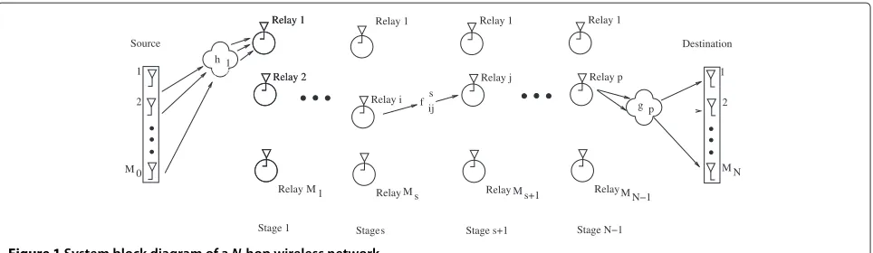
2 System model
Consider a multi-hop wireless network where a source ter-minal with M0 antennas wants to communicate with a
destination terminal with MN antennas viaN −1 relay
stages as shown in Figure 1. We refer to the multi-hop wireless network withN−1 relay stages as anN-hop net-work. Each relay in any relay stage has a single antenna;
Mndenotes the number of relays in thenth relay stage. It
Stage N−1 Relay 1
Relay 2
M 0
Relay Relay 2
M 1 h 1
Relay 1
Relay j
Relay
Relay M s M s+1
Relay 1
f ij s Relay i Source
Relay 1
M N Relay MN−1
Relay p
g p
Destination
Stage 1 1
2
Stage s Stage s+1
1
2 Relay 1
Figure 1System block diagram of aN-hop wireless network.
order of distance from the source towards the destination and any two relay nodes are chosen to lie in adjacent relay stages if they have sufficiently good SNR between them. In any practical setting, there will be interference received at any relay node of stagenbecause of the signals transmitted from relay nodes of relay stage 0,. . .,n−2 and n+ 2,. . .,N − 1. Due to relatively large distances between non-adjacent relay stages, however, this interfer-ence is quite small and we account for that in the additive noise term similar to [24]. More details are described in Remark 1.
As shown in Figure 1, the channel between the source and theith relay of the first stage of relays is denoted by hi =[h1i h2i . . . hM0i]T, i = 1, 2,. . .,M1, between the
jth relay of relay stage sand thekth relay of relay stage
s+1 byfjks, s = 0, 1,. . .,N −2, æ = 1, 2,. . .,Ms, k =
1, 2,. . .,Ms+1 and the channel between the relay stage N −1 and the th antenna of the destination byg = [g1g2 . . . gMN−1]T, =1, 2,. . .,MN. We assume that hi ∈ CM0×1,fjks ∈ C1×1,gl ∈ CMN−1×1are independent
and identically distributed (i.i.d.)CN(0, 1) entries for all
i,j,k,,s. We assume that themthrelay ofnthstage knows hi,fjks, ∀i, j, k,s = 1, 2,. . .,n−2, fjmn−1∀j, and the
des-tination knows hi,fjks,gl, ∀ i,j,k,l,s. We further assume
that all these channels are frequency flat and block fad-ing, where the channel coefficients remain constant in a block of time duration Tc and change independently
from block-to-block. We assume that the Tc is at least
max{M0,M1,. . .,MN−1}.
Remark 1.Duplexing:Duplexing is an important
con-sideration in multi-hop relay networks. For example, if relay stagenis receiving the signal from relay stagen−
1 and relay stage n + 1 is transmitting to relay stage
n + 2 simultaneously, then relay stage n will receive back flow of signals from relay stage n+ 1 that it has already transmitted. Since each relay stage uses an amplify and forward strategy, most of the power at relay stage
nwill then be used to retransmit signals that have been
transmitted before. A related paper [24] claims that back flow can be allowed with successive relay stages transmit-ting simultaneously without decreasing the diversity gain. That is true, however, in the limit of extremely large trans-mit power, and not applicable for any realistic transtrans-mit power level.
This problem is unique to greater than two-hop relay network and is not well understood. To avoid this situa-tion, a rate penalty of one-third is unavoidable for both full-duplex and half-duplex relay operation, where every third relay stage is switched on alternatively one at a time. For example, in first time slot communication hap-pens between relay stages 0− −1, 3 − −4, 6− −7,. . ., while in the second time slot communication happens between relay stages 1 − −2, 4 − −5, 7 − −8,. . ., in third time communication happens between relay stages 2 − −3, 5 − −6, 8 − −9,. . ., and so on, with periodic repetitions.
2.1 Problem formulation
Definition 1.(STBC) [30] A rate-L/TT×Ntdesign Dis
aT×Ntmatrix with entries that are complex linear
com-binations of L complex variables s1,s2,. . .,sL and their
complex conjugates. A rate-L/TT×NtSTBCSis a set of T×Ntmatrices that are obtained by allowing theL
vari-abless1,s2,. . .,sLof the rate-L/TT×NtdesignDto take
values from a finite subsetCf of the complex fieldC. The cardinality ofS= |Cf|L, where|Cf|is the cardinality ofC. We refer tos1,s2,. . .,sLas the constituent symbols of the
STBC.
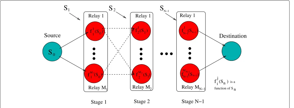
Definition 2.A DSTBC for an N-hop network
is a collection of STBCs {S0,S1,. . .,SN−1}, where S0
is the STBC transmitted by the source and Sn =
[φ1n(Sn−1) . . . φnMn(Sn−1)] is the STBC transmitted by
relay stagen, whereφnj(Sn−1)is the vector transmitted by
thejth relay of stagenwhich is a function ofSn−1, j =
0,. . .,Mn,n = 1,. . .,N−1. An example of a DSTBC is
S
S
S
Relay M2
Relay M1 function of Sn
1
Source Destination
Relay 1
2
Relay 1 Relay 1
S
0f1 1
fM11
fM2 2 2(S )
Stage 1 Stage 2
Relay MN−1
Stage N−1
N−1
f (S )0
1 1
fij(S )n is a fN−11
(S )
0 (S )1 f
MN−1
N−1
(S )N−2
(S )N−2
Figure 2An illustration Of the DSTBC design problem.
Definition 3.The diversity gain [1,3] of a DSTBCis defined as
d= − lim
E→∞
logPe(E)
logE ,
Pe(E) is the pairwise error probability using DSTBC ,
andEis the sum of the transmit power used by each node in the network.
The problem we consider in this article is to design DST-BCs that achieve the maximum diversity gain in anN-hop network. To identify the limits on the maximum possible diversity gain in anN-hop network, an upper bound on the diversity gain achievable with any DSTBC is presented next.
Theorem 1. The diversity gain d of DSTBC for
anN-hop network is upper bounded by min{MnMn+1},
n=0,1,. . .,N−1.
Proof. See Proposition 2.1 of [23].
Theorem 1 implies that the maximum diversity gain achievable in anN-hop network is equal to the minimum of the maximum diversity gain achievable between any two relay stages, when all the relays in each relay stage are allowed to collaborate. In the next section, we propose COSTBCs that are shown to achieve this upper bound on the diversity gain.
3 COSTBC
In this section, we introduce the COSTBC design for an
N-hop network. Before introducing COSTBCs, we need the following definitions.
Definition 4. With T ≥ Nt, a rate L/T T × Nt
STBC S is called full-rank or fully diverse or is said to achieve the maximum diversity gain if the differ-ence of any two matrices M1,M2 ∈ S is full-rank, i.e.,
minM1=M2,M1,M2∈Srank(M1−M2)=Nt.
Definition 5.A rate-L/K K × K STBC S is called an
OSTBC if the designDfrom which it is derived is orthog-onal, i.e.,DD∗=(|s1|2+ · · · + |sL|2)IK.
Definition 6. LetS be a rate-L/K K× K STBC. Then,
if the maximum likelihood (ML) decoding of S is such that each of the constituent symbols si, i = 1,. . .,L
of S can be decoded independently of sj ∀i = j i,j =
1,. . .,L, then S is called a single symbol decodable STBC.
Remark 2.OSTBCs are single symbol decodable STBCs
[25].
With these definitions we are now ready to describe COSTBCs for anN-hop network.
A COSTBC is a DSTBC where at each relay stage an OSTBC is transmitted, i.e.,Sn, n = 0, 1,. . .,N−1 is an
OSTBC. To construct COSTBC, the source transmits a rate-L/M0M0×M0OSTBCS0in a time slot of duration M0. The received signal y1k ∈ CM0×1at relay kof relay
stage 1 can be written as
y1k=E0S0hk+z1k, (1)
where E{tr(S∗0S0)} = M0, E0 is the power transmitted
is an OSTBC, using CSI, the received signal y1k can be
entries. Normalizingy˜1kby
In the second time slot of durationM1, relaykof relay
stage transmitst1k, constructed from the signal (3)
t1k= transmitted by each relay at any time instant isE1, i.e., E{t1†k t1k} =E1,A1k,B1kareM1×Lmatrices such that
A1k∗B1k = −Bk1∗A1k, andtrA1k∗(l)A1k(l)+Bk1∗(l)B1k(l) =1,
(5)
∀ k =1, 2. . .,M1, l = 1, 2,. . .L, whereA1k(l)andB1k(l)
denote the lth column of Ak and Bk, respectively, and
S1:=[A11s+B11s†. . .A1M1s+B 1 M1s
†] is an OSTBC.
Under these assumptions, theM1×1 received signal at
theithrelay of relay stage 2 is
S0. Thus, repeating the operations illustrated in (2), (3),
and (4), and using matricesAnk,Bnk, k = 1,. . .,Mn,n =
2,. . .,N−1 satisfying (5), an OSTBC is transmitted from each relay stage to construct the COSTBC.
Using COSTBCs, let the received signal at the kth antenna of the destination be
yNk =θEN−1SN−1ck+wNk, (7)
whereθ is such that the average power transmitted from the N −1th relay stage is EN−1, ck ∈ CMN−1×1 is the
equivalent channel vector between the source and thekth antenna of the destination, and wNk is the noise vector. Let yN :=[(y1N)T. . . (yNMN)T]T, c :=[c1T. . .cTMN]T, and w :=[(wN1)T. . . (wNMN)T]T, then with the ML decoding
whereR :=E{ww∗}is the noise covariance matrix. Note that if R is a scaled identity matrix, then the ML deci-sion rule (8) is equal to Lj=1minjf(sj), where f(sj)is a
function of sj that does not depend on sk,k = j, since
S∗N−1SN−1is a scaled identity matrix. Thus, the COSTBCs
are single symbol decodable ifRis a scaled identity matrix. With COSTBC, forj≥2, the noise vectorswjireceived at theith antenna of relay stagejare correlated fori =
1,. . .,Mj, since all the noise components of the signals
transmitted from the previous relay stagesnˆj1−1. . .nˆjM−1 j−1 have a contribution in all thewji,i=1,. . .,Mj. For
exam-ple in (6), w2i has contribution from nˆ1k (3) ∀ k =
1,. . .M1. Thus, in general, the noise covariance matrix
R with COSTBC is not a scaled identity matrix (not even diagonal), and hence the COSTBCs are not sin-gle symbol decodable. For a special case of N=2, and
M2=1, the noise covariance matrixRis diagonal,
how-ever, not a scaled identity matrix. Moreover, withN=2, andM2=1, an interesting property of COSTBC is that by
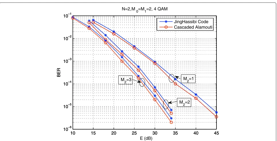
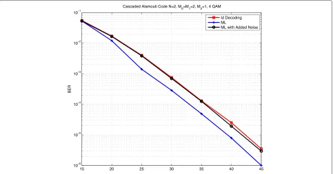
adding some channel coefficient-dependent noise terms to the received signal, the noise covariance matrix R can be made a scaled identity matrix as described in Appendix 2. Thus, compared to the ML detection of COSTBCs that entails joint decoding of symbols, by degrading the received signal and paying a penalty in terms of coding gain, COSTBCs are single symbol decod-able and hence have linear decoding complexity. A perfor-mance comparison with added noise term is illustrated in Figure 3.
Even though COSTBCs are not single symbol decod-able, we next show that with COSTBCs, maximum diver-sity gain can be achieved if the destination decodes all constituent symbols of COSTBCs independently of each other according to rule (10). Exploiting the orthogonality property of the OSTBCs transmitted by each relay stage, the received signal at the destination can be separated in terms of individual symbols transmitted by the source as follows. From (7), sinceSN−1is an OSTBC, similar to (2),
the received signal at thekth antenna of the destination can be transformed as
˜
yNk =θEN−1 ⎡ ⎢ ⎢ ⎢ ⎢ ⎣
|ck|2 0 0
0 . .. 0
0 0 |ck|2 ⎤ ⎥ ⎥ ⎥ ⎥ ⎦
s+zNk (9)
where s =[s1,s2, . . ., sL]T is the vector of the
con-stituent symbols of the OSTBC S0, and zNk is the
cor-related noise vector. Combining the transformed signals from allMN antennas, the received signal can be written
in terms of individual constituent symbols of the OSTBC S0, as
yN = Mn
k=1
cks+z,
10 15 20 25 30 35 40 45
10−6 10−5 10−4 10−3 10−2 10−1
E (dB)
BER
10 15 20 25 30 35 40 45
10−6 10−5 10−4 10−3 10−2 10−1
BER
N=2, M0=M1=2, 4 QAM
JingHassibi Code Cascaded Alamouti
M2=3 M2=1
M2=2
whereci = |ci|2andz =
Mn
k=1zNk()for=1, 2,. . .,L.
Thus, each symbolscan be decoded independently using the rule
s=arg min s ||y
N −
Mn
k=1
cks||2, (10)
even though this is not ML decoding. We consider this decoding rule to ensure linear decoding complexity and show that COSTBCs achieve maximum diversity gain with this rule.
Theorem 2.COSTBCs achieve the diversity gain upper
bound(Theorem 1) in anN-hop network with decoding rule (10).
Proof.See Appendix 1.
The basic idea behind the proof of Theorem 2 is to exploit the orthogonality of OSTBCs transmitted by each relay stage.
For the special case ofN=2 andM2=1, we next show
that the COSTBCs can be made single symbol decodable by degrading the received signal by adding some channel coefficient-dependent noise terms as discussed before.
Theorem 3.COSTBCs are single symbol decodable
STBCs after adding some channel coefficient-dependent noise terms to the received signals forN=2 andM2=1.
Proof.See Appendix 2.
Remark 3.CSI:We note that for decoding of COSTBCs, global CSI is required at the destination. The requirement of destination having global CSI regarding all the under-lying channels has been made in several recent related papers, including [23,24]. Actually, this is a common assumption made by all papers that consider amplify-and-forward protocol. Since mostly, only two-hop communi-cation is considered, the CSI requirement is somewhat limited compared to the case of multi-hop communica-tion, the topic of this paper and [22-24]. Acquiring such CSI in practice is a challenge, however, using techniques like Grassmannian codebooks, CSI about all channels can be acquired by the destination through the relay nodes by dedicating the start of time slots for training purposes. In particular, relay in stage 1 can get the CSI between source and itself by using pilots and channel estimation. There-after, by using Grassmannian codebooks it can forward the CSI it has gathered to the next relay stage in addition to sending pilots for the relays in the next stage to gather CSI between relay stages. Repeating this procedure all nodes can get the required CSI.
Another assumption about CSI we make for our code construction to work is that CSI is available at each relay node for channels preceding itself which is not required for other related works [22-24]. Since the CSI required at the destination for any amplify-and-forward protocol has to be transmitted through to the destination through the relays, CSI can safely be assumed to be available at each relay node as well. Thus, this is also not a limiting assumption.
Discussion: In this section, we constructed COSTBCs
by cascading OSTBCs at each relay stage. OSTBCs are cascaded at each relay stage by first separating each con-stellation symbol of the OSTBC transmitted from the pre-ceding relay stage, and then transmitting another OSTBC to the next relay stage. The proposed OSTBC cascading strategy is novel, and different than other approaches that use Alamouti code or OSTBC in a distributed manner [12,31].
We showed that the single symbol decodable property of OSTBCs is lost by cascading OSTBCs to construct COSTBCs. Using the orthogonality property of the OST-BCs, however, we showed that the maximum diversity gain can be achieved by COSTBCs even when each source transmitted symbol is decoded independently. Therefore, COSTBCs have decoding complexity that is linear in the number of symbols transmitted by source in one code-word, which is quite critical for practical implementa-tions. Since independent symbol decoding is not ML, COSTBCs entail an unavoidable coding gain loss, how-ever, we show that at least in terms of diversity gain there is no loss compared to ML decoding. We also showed that the COSTBCs are single symbol decodable for a two-hop wireless network N = 2 when the des-tination has only a single antenna M2 = 1, by adding
some channel coefficient-dependent noise terms to the received signal.
4 Explicit code constructions
In this section, we explicitly construct COSTBCs that achieve the maximum diversity gain in an N-hop net-work. The ingredient OSTBCs can be borrowed from [25,32,33], similar to [34]. We present examples of COST-BCs for N = 2, M0 = M1 = 2 using the Alamouti
code [26],N = 2, M0 = M1 = 4 using the rate-3/4
4 antenna OSTBC [25] andN = 2, M0 = M1 = 4
using the rate-3/4 4 antenna OSTBC and the Alamouti code.
Example 1.(Cascaded Alamouti code) We consider
N = 2,M0 = M1 = 2 case and letS0be the Alamouti
code given by Sala =
s1 s2 −s∗2 s∗1
constituent symbols of the Alamouti code. The 2 × 1 received signal at relaymis
form=1, 2. Transforming this in the usual way
1, 2 satisfy the requirements of (5). We call this the cas-caded Alamouti code.
Example 2. In this example, we consider the caseN=2,
M0=4,M1=4. We chooseS0to be the rate-3/4 OSTBC
for 4 transmit antennas given by
S0=
OSTBC as described above.
In both the previous examples, we constructed a COSTBC for the N = 2-hop case by repeatedly using the same OSTBC at both the source and the relay stage. Using a similar procedure, it can be seen that whenMi = Mj∀i,j=0, 1,. . .,N−1,i=jwe can construct
COST-BCs by using particular OSTBC for M0 antennas at the
source and each relay stage, e.g., if O is an OSTBC for
M0antennas, then by usingSn = O, n=0, 1,. . .,N−1
we obtain a maximum diversity gain achieving COSTBC. OSTBC constructions for different number of antennas can be found in [25]. In the next example, we construct COSTBC for M0 = 4 and M1 = 2 by cascading the
rate-3/4 4 antenna OSTBC with the Alamouti code.
Example 3.Let N = 2, M0 = 4, and M1 = 2. We
chooseS0to be the rate-3/4 4 antenna OSTBC (12) and
S1to be the Alamouti code. The COSTBC is constructed
as follows.
Let S0 given by (12) be the transmitted
rate-3/4 4 antenna OSTBC from the source. Then the received signal at relay node m, m = 1, 2 is Using CSI the received signal rm can be trans-formed into ˆrm, where rˆm := rˆm1 rˆm2 rˆm3 T =
These operations are repeated at the source and each relay stage in subsequent time slots. In the next time slot, signals3received in the previous time slot ands1received
in the current time slot is transmitted from relay stage 1 to the destination. Clearly, the relay stage transmits an Alamouti code which is an OSTBC and hence leads to a COSTBC construction forM0=4,M1=2.
source antenna and relay node configurations by suitably adapting different OSTBCs.
5 Simulation results
In this section, we provide simulation results to illus-trate the bit error rates (BERs) of COSTBCs for 2- and 3-hop networks. In all the simulation plots, E denotes the total power used by all nodes in the network, i.e.,
E0+nN=−11MnEn=Eand the additive noise at each relay
and the destination is complex Gaussian with zero mean and unit variance. By equal power allocation between the source and each relay stage we mean E0 = MnEn =
E
N, ∀n=1,. . .,N−1.
In Figure 4, we plot the BERs of a cascaded Alam-outi code and the comparable DSTBC from [3] with 4 QAM modulation for N = 2, M0 = M1 = 2, and M2 = 1, 2, 3 with equal power allocation between the
source and all the relays. It is easy to see that both the cas-caded Alamouti code and the DSTBC from [3] achieves the maximum diversity gain of the 2-hop network, how-ever, COSTBCs require 1 dB less power than the DSTBCs from [3], to achieve the same BER. The improved BER performance of COSTBCs over DSTBCs from [3] is due to fact that with COSTBCs, each relay coherently com-bines the signal received from the previous relay stage before forwarding it to the next relay stage, while no such combining is done in [3]. Note that, however, DST-BCs from [3] do not need CSI at any relay, in contrast to COSTBCs which use CSI for transforming the signal and transmitting an OSTBC. To illustrate the loss with
independent decoding (10) with respect to ML decoding, forN = 2 and M2 = 1, in Figure 3, we plot the BER
performance of cascaded Alamouti codes with ML decod-ing, with independent decoding (10), and adding channel coefficient-dependent noise for which the COSTBC is single symbol decodable. We observe that even though there is a sufficient gap between ML and non-ML decod-ings, there is a negligible difference between indepen-dent decoding (10) and ML single symbol decoding with added noise.
We also compare the BER performance of COSTBC with perfect and imperfect CSI in Figure 5 for a 2-hop net-work with number of destination antennas M2 = 1, 2.
Each relay uses channel estimation with the help of pilots to gather the necessary CSI from the source to itself. Then each relay uses a 16-bit Grassmannian codebooks [35] for relaying the CSI between source and relay it has estimated, in addition to sending pilots for the destination to get the CSI between each relay and destination. We notice that even though there is a performance loss with imperfect CSI, however, its not too significant.
Next, we plot the BER curves forN=2,M0=M1=4,
andN = 2,M0 = 4, M1 = 2 configurations in Figures 6
and 7 with differentM2and using equal power allocation
between the source and the relay stage. For theM0 = M1 = 4 case, we use the cascaded rate-3/4 4 antenna
OSTBC and for theM0 = 4, M1 =2 case we use a
rate-3/4 4 antenna OSTBC at the source and the Alamouti code across both the relays as discussed in Section 4. From Figures 6 and 7, it is clear that both these codes achieve
Figure 5BER comparison of cascaded Alamouti code with perfect and imperfect CSI forN=2-hop network.
the maximum diversity gain for the respective network configurations.
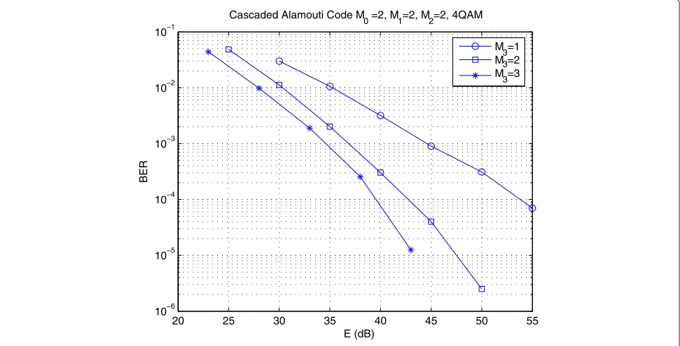
Finally, in Figure 8, we plot the BERs of a cascaded Alamouti code with N = 3-hop network where M0 = M1 = M2 = 2 with M3 = 1, 2, 3, and the cascaded
Alamouti code is generated by repeated use of the Alam-outi code by each relay stage with equal power allocation
between the source and the relay stages. In this case also, it is clear that the cascaded Alamouti code achieves the maximum diversity gain but there is an SNR loss compared toN = 2 case, because of the noise added by one extra relay stage.
From all the simulation plots, it is clear that COST-BCs require large transmit power to obtain reasonable
4 6 8 10 12 14 16 18 20 22
10−5 10−4 10−3 10−2 10−1 100
E (dB)
BER
Cascaded rate 3/4 OSTBC M0 =4, M1=4, 4QAM
M
2=1
M2=2
12 14 16 18 20 22 24 26 28 30 10−5
10−4 10−3 10−2 10−1
E (dB)
BER
Cascaded rate 3/4 OSTBC with Alamouti M
0 =4, M1=2, 4QAM
M2=1
M
2=2
Figure 7Cascaded rate 3/4 4 antenna OSTBC with Alamouti Code forM0=M1=4.
BERs with multi-hop wireless networks. This is a com-mon phenomenon across all the maximum diversity gain achieving DSTBCs for multi-hop wireless networks that use AF [3,5,9]. With AF, the noise received at each relay gets forwarded towards the destination and limits the received SNR at the destination, however, without using AF it is difficult to achieve the maximum diversity gain in a multi-hop wireless network.
6 Conclusion
In this article, we designed COSTBCs that achieve the maximum diversity gain in a multi-hop wireless network with low decoding complexity. We then gave an explicit construction of COSTBCs for various numbers of source, destination, and relay antennas. The only restriction that COSTBCs impose is that the source and all the relay stages have to use an OSTBC. It is well known that high rate
20 25 30 35 40 45 50 55
10−6 10−5 10−4 10−3 10−2 10−1
E (dB)
BER
Cascaded Alamouti Code M0 =2, M1=2, M2=2, 4QAM
M
3=1
M3=2 M3=3
OSTBCs do not exist; therefore, the COSTBCs have rate limitations. For future work it will be interesting to see whether the OSTBC requirement can be relaxed with-out sacrificing the maximum diversity gain and minimum decoding complexity of the COSTBCs.
Appendix 1
We prove Theorem 2 using induction. First we show that COSTBCs achieve the maximum diversity gain forN=2, and then extend the result for ak-hop network, wherekis any arbitrary natural number.
The outage probabilityPout(R)is defined asPout(R) := P(I(s;r)≤R), where s is the input and r is the out-put of the channel and I(s;r)is the mutual information between s andr [36]. Let dout(r) be the SNR exponent
of Pout with rate of transmission Rscaling as rlogSNR,
i.e., logPout(rlogSNR) =. SNR−dout(r). Then, ifPe(SNR) =. SNR−d(r), then from [29], and the compound channel argument [24],Pout(rlogSNR)=. Pe(SNR), d(r)=. dout(r).
Therefore, to compute d(r), it is sufficient to compute
dout(r). In the following, we compute dout(r) for the
COSTBC with a 2-hop network.
For the 2-hop network, similar to (2), from (19), the received signal at any receive antenna of the destination can be separated in terms of the individual constituent symbols of the OSTBC transmitted by the source. Similar to (2), from (19), separating the constituent symbols ofS0,
letyjbe the received signal at thejth antenna of the desti-nation corresponding tos, theth, l=1, 2,. . .,Lsymbol transmitted from the source. Thenyjcan be written as
yj=θE1
whereθ is the normalization constant so as to ensure the power constraint ofE1for the relay stage 1, andzj is the additive white Gaussian noise (AWGN) with zero mean andσj2 variance. Note thatzj’s are not independent for
j = 1,. . .,M2. Adding the received signal corresponding
tosfrom all the antennas of the destination of the 2-hop network, we get dent, any linear combination ofzjl’s is Gaussian, therefore
z is CN(0,σ2) distributed for some σ2. Note that σ2 depends on the channel coefficients, however, as shown in Theorem 2.3 of [24],zis white in the scale of interest and without loss of generalityz can be modeled asCN(0, 1), i.e., independent of channel coefficients in the outage analysis. ability of a single input single output system which can be computed easily using [29], and is given by
P
the diversity gain upper bound (Theorem 1). Thus, we have shown that COSTBCs achieve the maximum diver-sity gain in a 2-hop network. Next, using induction, we prove the result for anyk-hop network.
Assume that the result is true for a k-hop network
(k ≥ 2), and we will prove that it is true for ak+1-hop network. Similar to 2-hop case, for ak-hop network also, at the destination, the received signal can be separated in terms of the individual constituent symbols of the OSTBC transmitted by the source. Thus, the received signal at the destination of the k-hop network corresponding to the signalscan be written as
yk =θk−1Ek−1 Mk
i=1
cis+z, (15)
whereθk−1is the normalization constant so as to ensure
the average power constraint of Ek−1 is satisfied at the
relay stagek−1,sis theth,=1, 2,. . .,Lsymbol trans-mitted from the source,ciis the channel gain experienced
by s at the ith antenna of the destination, andzl is the
AWGN with varianceσk2.
Now we extend thek-hop network to ak+1-hop net-work by assuming that the actual destination to be one more hop away and using the destination of thek-hop case as thekth relay stage withMkrelays by separating theMk
to thek-hop case, the received signal at the destination of thek+1-hop can also be separated in terms of individ-ual constituent symbols of the OSTBC transmitted by the source, which is given by
yk+1=θkEk
whereθk is a constant to ensure the power constraint of Ek in thek+1-hop network,gijis the channel between
the ith relay of relay stage k and thejth antenna of the destination, andnlis the AWGN with varianceσk2+1. Let
Recall from induction hypothesis that the diversity gain of COSTBCs with channel ci,∀ i (15) is α :=
min#min{MnMn+1}, Mk−1 $
, n = 0, 1,. . .,k − 2, by restricting the destination of the k-hop network to have only single antenna, and with channel Mk
i=1ci is
min{MnMn+1}, n = 0, 1,. . .,k−1, respectively. Thus,
if the diversity gain of COSTBCs with channel qi (17)
is min#min{MnMn+1}, Mk−1,Mk+1 $
n = 0, 1,. . .,k−
2, then, since Mk+1
j=1 |gij|2 are independent ∀ i, it
fol-lows that the diversity gain of COSTBCs with channel
Mk
i=1qiis min{MnMn+1}, n=0, 1,. . .,k. Next, we show
that the diversity gain of COSTBCs with channel qi is
min#min{MnMn+1}, Mk−1,Mk+1 $
, n=0, 1,. . .,k−2. To compute the diversity gain of COSTBCs with chan-nelqi(17), we use the outage probability formulation [29]
as follows. Letσ2be the variance ofni(17),σ2 = σ2
k+1 M2k ,
however, as before using Theorem 2.3 of [24]niis white
in the scale of interest, and can be modeled asCN(0, 1). By induction hypothesis, the diversity gain of COSTBCs withciisα, i.e.,
wherek4is a constant. Thus,
Pout(rlogSNR)≤P
SinceZis a gamma distributed random variable with PDF
e−zzMk+1−1
Mk+1−1! , the first term inPout(rlogSNR)expression can be found in [29] and is given by PZ≤SNR−(1−r) =. SNR−Mk+1(1−r). Now we are left with computing the sec-ond term which can be done as follows.
% ∞
Thus, from (18) it follows that
Pout(rlogSNR)=. SNR−Mk+1(1−r)+SNR−α(1−r) .
=SNR−min{Mk+1,α}(1−r).
Using the definition of diversity gain, it follows that the diversity gain of COSTBCs with channelqi is equal
of COSTBCs with the received signal model (16) is min{αMk,MkMk+1}. Note that the upper bound on the diversity gain
(Theorem 1) is also min{αMk,MkMk+1}, and hence we conclude that the COSTBCs achieve the maximum diversity
gain in anN-hop network.
Appendix 2
In this section, we prove that COSTBCs have the single symbol decodable property forN=2 andM2=1.
LetS0be the transmitted OSTBC from the source, ands =[s1,. . .,sL]T be the vector of the constituent symbols of
S0. Then from (3), using CSI, the received signaly1k at thekth relay of relay stage 1 can be transformed intoyˆ1k, where ˆ
y1k =
E0H1ks+ ˆn1k, whereH1kis defined in (2), and the entries ofnˆkare independent andCN(0, 1)distributed. ForN=2,
andM2 =1, from (6), the received signal at the destination can be written asy21=[t11t12 . . . t1M1]g1+z 2
1, wheret1kis
the transmitted vector from relayk(4) of relay stage 1. The received signaly21can also be written as
y21 =
E0E1M
Lγ S1 Mm=01|hm1|2g11
M0
m=1|hm2|2g21 . . .
M0
m=1|hmM1|2gM11
C
T
+
E1M1
Lγ [A1nˆ1+B1nˆ †
1A2nˆ2+B2nˆ†2 . . . AM1nˆM1+BM1nˆ †
M1]g1+z 2 1
w
, (19)
whereS1=[A11s+B11s†A21s+B12s† . . . AM1s+BM1s
†].
LetR=E{ww∗}be the noise covariance matrix. Note that
R= E1M1
Lγ ⎡ ⎢ ⎢ ⎢ ⎣
g∗1D1g1 0 . . . 0
0 g∗1D2g1 . . . 0
0 . . . . .. 0
0 . . . 0 g∗1DM1g1
⎤ ⎥ ⎥ ⎥ ⎦+IM1,
whereDj = (A1jA1j∗+B1jB1j∗)is a diagonal matrix whose diagonal entries are either zero or one sinceAjandBjare
constituents of an OSTBC, and the number of ones inDjis equal tok, ifAjandBjare constituents of a ratek/nOSTBC.
Note that the locations of non-zero entries ofDjcan be different for differentj’s, and henceRis not necessarily a scaled
identity matrix. Therefore, because of the non-diagonal structure ofR−1, the ML decoding metric (8) cannot be split in several terms, where each term is a function of only one of the constituent symbols ofS1. Therefore in general,
COSTBCs are not single symbol decodable. The problem can, however, be fixed easily by adding an additional channel coefficient-dependent noise vector to the received signal at the receiver as follows.
Let1j=diag(Dj),1j∈ {0, 1}M1×1, and1cj be the complement of1j, i.e., any entry of1cj is 1 if that entry of1jis 0, and
vice versa. Letζj=1cj[|g11|2|g21|2. . . |gM11|2]T, anda=
E1M1
Lγ [ √
ζ1u1√ζ2u2. . .
ζM1uM1]T, whereui,i=1,. . .,M1 are i.i.d. withCN(0, 1)distribution. Then to make the noise covariance a scaled identity matrix,acan be added to the received signal at the destinationy21. Withya=y21+a, the noise vectorwa=w+a, and the covariance matrix
Rwa=E{nan∗a} = E1M1
Lγ ⎡ ⎢ ⎢ ⎢ ⎣
|g1|2 0 . . . 0 0 |g1|2 . . . 0 0 . . . . .. 0
0 . . . 0 |g1|2
⎤ ⎥ ⎥ ⎥ ⎦+IM1,
which is a scaled identity matrix. Hence, usingya(instead ofy) to decodeS1, the ML decoding metric (8) splits inL
different terms, where each term is a function of only one of the constituent symbols ofS0, and the COSTBC is single
Competing interests
The authors declare that they have no competing interests.
Acknowledgements
This material is based upon work supported by the Army Research Laboratory Labs W911NF-10-1-0420 and by the National Science Foundation
NSF-CCF-1218338.
Author details
1School of Technology and Computer Science, Tata Institute of Fundamental
Research, Mumbai 400005, India.2Wireless Networking and Communications
Group, Department of Electrical and Computer Engineering, The University of Texas at Austin, 1 University Station C0803, Austin, TX 78712–0240, USA.
Received: 20 November 2012 Accepted: 18 March 2013 Published: 25 April 2013
References
1. V Tarokh, H Jafarkhani, A Calderbank, Space-time block coding for wireless communications: performance results. IEEE J. Sel. Areas Commun.17(3), 451–460 (1999)
2. J Laneman, G Wornell, Distributed space-time-coded protocols for exploiting cooperative diversity in wireless networks. IEEE Trans. Inf. Theory.49(10), 2415–2425 (2003)
3. Y Jing, B Hassibi, Diversity analysis of distributed space-time codes in relay networks with multiple transmit/receive antennas. EURASIP J. Adv. Signal Process.2008, Article ID 254573 (2008)
4. R Nabar, H Bolcskei, F Kneubuhler, Fading relay channels: performance limits and space-time signal design. IEEE J. Sel. Areas Commun. 22(6), 1099–1109 (2004)
5. Y Jing, B Hassibi, Distributed space-time coding in wireless relay networks. IEEE Trans. Wirel. Commun.5(12), 3524–3536 (2006)
6. S Yang, J-C Belfiore, Optimal space time codes for the MIMO amplify-and-forward cooperative channel. IEEE Trans. Inf. Theory. 53(2), 647–663 (2007)
7. G Susinder Rajan, B Sundar Rajan, inProceedings of IEEE Information Theory Workshop. A non-orthogonal distributed space-time coded protocol, Part-I: signal model and design criteria (IEEE, Punta del Este, Uruguay, October 22–26 2006), pp. 385–389
8. G Susinder Rajan, B Sundar Rajan, inProceedings of IEEE Information Theory Workshop. A non-orthogonal distributed space-time coded protocol, Part-II: code construction and DM-G tradeoff (IEEE, Punta del Este, Uruguay, October 22–26 2006), pp. 488–492
9. F Oggier, B Hassibi, inIEEE International Symposium on Information Theory, 2006. An algebraic family of distributed space-time codes for wireless relay networks (IEEE, Punta del Este, Uruguay, July 2006), pp. 538–541 10. T Kiran, B Rajan, inIEEE International Symposium on Information
Theory,2006. Distributed space-time codes with reduced decoding complexity, (July 2006), pp. 542–546
11. P Elia, P Vijay Kumar, Approximately universal optimality over several dynamic and non-dynamic cooperative diversity schemes for wireless networks, available at http://arxiv.org/pdf/cs.it/0512028,
December 7, 2005
12. Y Jing, H Jafarkhani, Using orthogonal and quasi-orthogonal designs in wireless relay networks. IEEE Trans. Inf. Theory.53(11), 4106–4118 (2007) 13. G Susinder Rajan, B Sundar Rajan, inIEEE International Symposium on
Information Theory. Algebraic distributed space-time codes with low ML decoding complexity (IEEE, Nice, France, June 24–29 2007),
pp. 1516–1520
14. Z Yi, I-M Kim, Joint optimization of relay-precoders and decoders with partial channel side information in cooperative networks. IEEE J. Sel. Areas Commun.25(2), 447–458 (2007)
15. J Harshan, B Rajan, High-rate, single-symbol ML decodable precodedDSTBCs for cooperative networks. IEEE Trans. Inf. Theory. 55(5), 2004–2015 (2009)
16. J Harshan, B Rajan, A Hjorungnes, inIEEE International Symposium on Information Theory Proceedings (ISIT), 2010. Training-symbol embedded, high-rate complex orthogonal designs for relay networks (IEEE, Austin TX, USA, June 2010), pp. 2233–2237
17. D Sreedhar, A Chockalingam, B Rajan, inIEEE International Symposium on Information Theory, 2008. ISIT 2008. High-rate, single-symbol decodable
distributed STBCs for partially-coherent cooperative networks, (July 2008), pp. 2538–2542
18. D Sreedhar, A Chockalingam, B Rajan, Single-symbol ML decodable distributed STBCs for partially-coherent cooperative networks. IEEE Trans. Wirel. Commun.8(5), 2672–2681 (2009)
19. K Srinath, B Rajan, inIEEE Information Theory Workshop (ITW). Single real-symbol decodable, high-rate, distributed space-time block codes (IEEE, Dublin Ireland, 2010), pp. 1–5
20. T Duong, H Tran, inIEEE Radio and Wireless Symposium, 2008. Distributed space-time block codes with amicable orthogonal designs (IEEE, Orlando, FL, USA, January 2008), pp. 559–562
21. F Verde, A Scaglione, inIEEE International Conference on Acoustics Speech and Signal Processing (ICASSP). Randomized space-time block coding for distributed amplify-and-forward cooperative relays (IEEE, Dallas,TX, USA, 2010), pp. 3030–3033
22. F Oggier, B Hassibi, Code design for multihop wireless relay networks. EURASIP J. Adv. Signal Process.2008, Article No. 68 (2008)
23. S Yang, J Belfiore, Diversity of MIMO multihop relay channels, available on http://arxiv.org/abs/0708.0386, August 2007
24. K Sreeram, S Birenjith, P Kumar, Dmt of multihop networks: end points and computational tools. IEEE Trans. Inf. Theory.58(2), 804–819 (2012) 25. V Tarokh, H Jafarkhani, A Calderbank, Space-time block codes from
orthogonal designs. IEEE Trans. Inf. Theory.45(5), 1456–1467 (1999) 26. S Alamouti, A simple transmit diversity technique for wireless
communications. IEEE J. Sel. Areas Commun.16(8), 1451–1458 (1998) 27. R Vaze, R Heath, inProceedings of the Information Theory and Applications,
2008. Maximizing reliability in multi-hop wireless networks with cascaded space-time codes (IEEE, San Diego, CA, USA, January–February 2008) 28. R Vaze, R Heath, inIEEE International Symposium on Information Theory,
2008. ISIT 2008. Maximizing reliability in multi-hop wireless networks, (July 2008), pp. 11–15
29. L Zheng, D Tse, Diversity and multiplexing: a fundamental tradeoff in multiple-antenna channels. IEEE Trans. Inf. Theory.49(5), 1073–1096 (2003)
30. B Sethuraman, B Rajan, V Shashidhar, Full-diversity, high-rate space-time block codes from division algebras. IEEE Trans. Inf. Theory.
49(10), 2596–2616 (2003)
31. KR Kumar, G Caire, Coding and decoding for the dynamic decode and forward relay protocol. IEEE Trans. Inf. Theory.55(7), 3186–3205 (2009) 32. W Su, S Batalama, D Pados, On orthogonal space-time block codes and
transceiver signal linearization. IEEE Commun. Lett.10(2), 91–93 (2006) 33. W Su, X-G Xia, K Liu, A systematic design of high-rate complex orthogonal
space-time block codes. IEEE Trans. Commun.8(6), 380–382 (2004) 34. F Verde, in5th International Symposium on Communications Control and
Signal Processing (ISCCSP), 2012. Design of randomized space-time block codes for amplify-and-forward cooperative relaying (IEEE, Kyoto, Japan, May 2012), pp. 1–5
35. D Love, RW Heath Jr, T Strohmer, Grassmannian beamforming for multiple-input multiple-output wireless systems. IEEE Trans. Inf. Theory. 49(10), 2735–2747 (2003)
36. T Cover, J Thomas,Elements of Information Theory(Wiley, New York, 2004)
doi:10.1186/1687-1499-2013-113