The track finding algorithm of the Belle II vertex detectors

The track finding algorithm of the Belle II vertex detectors

Tadeas Bilka1_{, Nils Braun}2_{, Giulia Casarosa}3,4,5_{, Oliver Frost}6_{, Rudolf Frühwirth}7_, Thomas Hauth2_{, Martin Heck}2_{, Jakub Kandra}1_{, Peter Kodys}1 _{Peter Kvasnicka}1_, Jakob Lettenbichler7_{, Thomas Lück}3,4,8,a_{, Thomas Madlener}7_{, Felix Metzner}2_{, Moritz} Nadler7_{, Benjamin Oberhof}3,4_{, Eugenio Paoloni}3,4_{, Markus Prim}2_{, Martin Ritter}9_{, Tobias} Schlüter, Michael Schnell10_{, Bjoern Spruck}5_{, Viktor Trusov}6_{, Jonas Wagner}2_{, Christian} Wessel10_{, and Michael Ziegler}2

1_{Charles University, Prague (Czech Republic)}

2_{IEKP, Karlsruhe Institute of Technology, Karlsruhe (Germany)}

3_{I.N.F.N. sezione di Pisa, Pisa (Italy)} 4_{Università di Pisa, Pisa (Italy)}

5_{Institut für Kernphysik Johannes Gutenberg-Universität, Mainz (Germany)}

6_{Deutsches Elektronen-Synchrotron, Hamburg, (Germany)} 7_{Institute of High Energy Physics, Vienna (Austria)}

8_{Scuola Normale Superiore di Pisa, Pisa (Italy)}

9_{Excellencecluster Universe, Ludwigs-Maximillians-University (Germany)}

10_{Physikalisches Institut Rheinische Friedrich-Wilhelms-Universität, Bonn (Germany)} 11_{Excellencecluster Universe, Ludwigs-Maximillians-University, Munich (Germany)}

Abstract.The Belle II experiment is a high energy multi purpose particle detector op-erated at the asymmetrice+e−- collider SuperKEKB in Tsukuba (Japan). In this work we describe the algorithm performing the pattern recognition for inner tracking detector which consists of two layers of pixel detectors and four layers of double sided silicon strip detectors arranged around the interaction region. The track finding algorithm will be used both during the High Level Trigger on-line track reconstruction and during the off-line full reconstruction. It must provide good efficiency down to momenta as low as 50 MeV/c where material effects are sizeable even in an extremely thin detector as the VXD. In addition it has to be able to cope with the high occupancy of the Belle II de-tectors due to the background. The underlying concept of the track finding algorithm, as well as details of the implementation are outlined. The algorithm is proven to run with good performance on simulatedΥ(4S)→B_B¯events with an efficiency for reconstructing tracks of above 90% over a wide range of momentum.

1 Introduction

Belle II is a multipurpose detector which will be operated at the asymmetric B-Factory SuperKEKB (Japan). The unprecedented instantaneous luminosity of up to 8×1035_cm−2_s−1 _{provided by the} accelerator together with the soft spectrum of the charged particles to be traced (typical momentum

350 MeV/c and with the high occupancy (1.5%) foreseen in the inner silicon layers will challenge the sub-detectors of Belle II and the track finding algorithms.

Track position information close to the interaction point is provided by the vertex detector (VXD) which consists of 2 layers of pixel detectors (PXD) and 4 layers of double sided silicon strip vertex detectors (SVD) whose overall thickness and dead material is kept at a minimum to reduce the effects of multiple Coulomb scattering.

The track finding code for the VXD of Belle II implements in an efficient way the Sector Map concept originally proposed by Rudolf Frühwirth and originally implemented by Jakob Lettenbich-ler [1].

The typical event recorded by the VXD will be dominated by random hits produced by beam background (order of 500 pixels hit per event per sensor on the inner layer of the PXD, 20 GByte/s required to readout the whole PXD). In this harsh environment the pattern recognition algorithm for the VXD has to be capable to efficiently and quickly recognize the 11 long lived charged particles emerging as decay products of a typicalΥ(4S) event.

The track finding algorithm presented here will be used both during the final reconstruction of the event and during the fast reconstruction occurring on the High Level Trigger (HLT) for the definition of the Regions Of Interest on the PXD sensors used to reduce the PXD data stream to a manageable level [2]. This latter task put tight constraints on the reliability and time consumption of the track finding algorithm since an eventual crash or malfunction of the HLT process will immediately translate in a permanent loss of data and since the time left for the silicon vertex identification is in the ball park of a few milli-seconds per event.

This paper presents the main concepts of the algorithm, some details of its implementation to-gether with its current performances.

2 The Belle II detector and the inner tracking devices

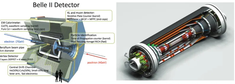
The Belle II detector is described in detail elsewhere [3]. Here are described only the inner silicon tracking devices for which the track finding algorithm is designed. The inner tracking detector consists of two layers of DEPFET pixel detectors (PXD) [4], which are arranged around the beam at the radii of 14 mm and 22 mm from the interaction point. Its inner layer consists of 8 sensors with dimension 15×90 mm2_{while its outer layer consist of 12 modules of the size of 15×123 mm}2_{. The silicon has} been thinned down to 75μm to reduce the radiation length. The angular acceptance starts at a polar angle of 17◦in the forward direction and ends to 150◦. The size of the pixels is 50×50μm2_{for the} inner layer and 50×75μm2_{for the outer layer, respectively.}

The PXD is surrounded by the Silicon Vertex Detector (SVD) [5] which consists of 4 layers of double sided silicon strip detectors positioned at radii of 38 mm, 80 mm, 115 mm, and 140 mm from the interaction point. The sensors have readout pitches in ther−φ-direction (p-Side) between 50μm and 75μm, and between 160μm and 240μm in thez-direction (n-Side). To increase the resolution of the reconstructed position a floating strip is present in-between two readout strips. The sensors are arranged in ladders which are made of 2, 3, 4, and 5 sensors per ladder for layer 3, 4, 5, 6 (counting starts from the first PXD layer), respectively. The number of ladders per layer is 7, 10, 12, 16 going from the inner to the outer layer of the SVD, respectively. To reduce the amount of material in the forward region the shape of the ladders in layers 4, 5, and 6 are such to form a peculiar “lamp shade” geometry (cfr. Fig. 1 ) in which the forward sensors for layers 4, 5, and 6 are trapezoids slanted with respect to the beam pipe.

(a) The Belle II detector. (b) Schematic of the Vertex detectors.

Figure 1: Shown is a schematic of the Belle II detector (a), and a schematic of the vertex detectors of Belle II (b).

3 Track finding concept

Due to the nature of theB-meson decays the track finding has to deal with very low momentum

par-ticles. The most probable momentum of the long lived decay products of theBis around 350 MeV/c

moreover the track finding algorithm must efficiently work down to momenta of around 50 MeV/c

for which the only tracking informations are coming from the VXD. An additional challenge is the extremely high background from by the pairs productions processe+e− → e+e−e+e− whose large cross section will rise the occupancy in the PXD inner layer to 1.5 %. The concept of the track finding

for the Belle II experiment was chosen to efficiently cope with these requirements in this

unprece-dently harsh environment: track seeds formed using SVD and DCH hits are used to define Regions Of Interest (ROI) on the PXD. Just the PXD hits inside these ROIs together with additional PXD clusters selected by a Neural Network according to their position, charge, multiplicity and shape will be written on disk for the final event reconstruction.

Additional ROIs will be provided by the DATCON (an FPGA based tracking device that will use only SVD hits and that will run in parallel with respect to the HLT) that is described in details in another proceeding of this very same conference.

The finding of track candidates works in several steps which will be sketched in the following sections. These steps are, in this very order, the combination of two hits to produce segments, the combination of segments into track candidates, the quality estimation of the track candidates and fi-nally the removal of random combinations of hits (that is, fake tracks) from the list of track candidates to be used for the final Kalman fit.

The implementation of the track finding algorithm for the Belle II vertex detectors is implemented in C++11 and is part of the Belle II analysis software framework [6].

3.1 The sector map concept.

Carlo (MC) tracks the geometry of the detector. This is particularly appealing in Belle II since the VXD lacks trivial geometrical discrete symmetry.

The training sample should represent the momentum spectrum and particle type composition (due to differences in interactions with the material for different particle types) expected for the actual data sample. For the results presented in this document a training sample of simulatedΥ(4S)→BB¯events have been used.

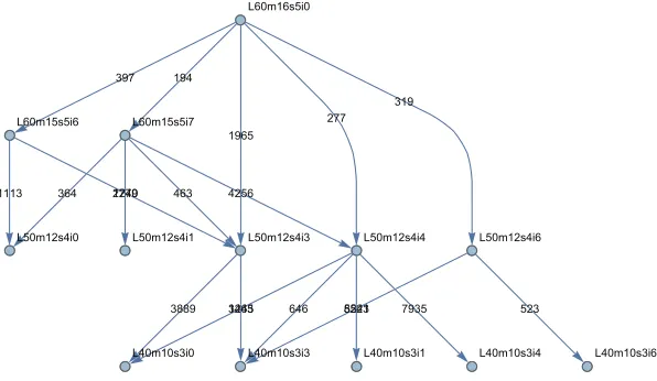
At the heart of the concept of sector map is the partition of the sensors surface in SectorsSi.

Each sectorSi is connected in a so called “friendship relationFi j” to a sectorSj if trajectories are

passing throughSiandSjwithout crossing any other sector in between. If we limit our analysis to

the outgoing arm of the track coming from the interaction point, it turns out that the set{Fi j}defines a

cycle free graph on the set of nodes{Si}(that is,{Si}is the set of nodes and{Fi j}is the set of edges).

Moreover the curvilinear coordinate on the trajectories defines a natural direction of each edge of this graph, so that in the end the trajectories induce on{Si}a directed sortable graph structure that will be

exploited in the following. A subset of this graph is represented in Fig. 2.

1965

277 319 397 194

3889 3463346312454 646 85238523524152 7935 523 2279

1113 364 174022 463 4256 L60m16s5i0

L50m12s4i3 L50m12s4i4 L50m12s4i6 L60m15s5i6 L60m15s5i7

L40m10s3i0 L40m10s3i3 L40m10s3i1 L40m10s3i4 L40m10s3i6 L50m12s4i0 L50m12s4i1

Figure 2: A subset of the graph defined by friendship relations among sectors. The format of the sector name is Lllmxxsyyizzwherellis the layer and sub layer id,xxis the module number,yy is the sensor number andzzis the sector number. The number on the directed edge corresponds to the number of tracks in the training samples connecting the two sectors.

SectorSiis defined as outer with respect toSjif the trajectories connecting them are going from Sj toSi. With these natural definition the outer sectors are on the geometrical outer layers of the

tracking device. A sample of MC tracks are used for defining the friend relations among sectors. The MC events used for the definition of the friend relations are produced with a full Geant 4 detector simulation. In the current version of the code both the number and the position of the corners of the sectors can be set individually for each sensor, separately for u and v-direction. This allows to chose a different setting for the sectors in different detector regions for example to cope with different level of backgrounds found in these regions. The results presented in the following are obtained partitioning the sensors in 9 sectors arranged in a 3×3 array.

views of a sensor are preliminary combined in a single Space Point (SP) which represents the 3D position in the global coordinates system. The SPs are stored in a container whose access key is the SectorSi on which the SP belongs. A sector containing one or more SP is defined as an “active

sector”.

The next step is to find compatible combinations of two hits (in the following called segments). A loop over the active sectors is performed and for each hit belonging to a sectorSithe second hit is

searched only in active sectorsSjwhich are friends of the sectorSi. The approach of considering only

pairs of friends sectors drastically reduces the number of possible two-hit combinations moreover, since the average occupancy of the sector is order one SP/ sector under pessimistic background assumptions just in the inner SVD layer, the computational complexity of this step is still linear with the number of SP (at least up to reasonable background running conditions).

For each friendship relationFi j a set of geometrical requirements is defined to be fulfilled by

the segmentsto be accepted and used in the next steps of the reconstruction. The geometrical re-quirements are expressed as a set of inequalities on several geometrical variablesv_α(s). Due to the complicated geometry of the detector it is not sufficient to set the limits for thev_α(s) globally. For that reason the upper and lower bound for eachv_α(s) are set individually for each friendship relation. The inequalities used so far have the simple form mini jα ≤vα(s)≤ maxi jαwhere the min and max values allowed forv_α(s) do depend on the indexes of the two friends sectorsiand jand their value is tuned using the training sample used also for the definition of the sector connection. The currently implemented geometrical variables for the characterization of the segment are:

• the squared 2D distance between the two SPs in the x-y-plane (perpendicular to the B-field),

• the squared distance between the two SPs in 3D,

• the distance between the two SPs in the direction of the B-field,

• the angle between the direction of the B-field and the direction defined by the two SPs,

• and the normalized distance in 3D between the two SPs.

The segments fulfilling these requirements are accepted and stored in a container whose access key is the friendship relationFi j whereSi (Sj) is the sector containing the outer (inner) SP of the

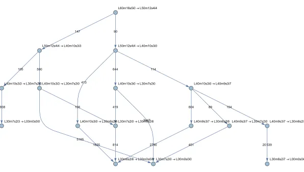
segment. A friendship relation is defined active if there is at least one segment associated to it. The accepted segments are passed to the next step in which they are combined into SP tripletst. For this step the graph structure induced by trajectories on the set{Fi j}is again exploited. A graph is built in

which the nodes are the set of friendship relation{Fi j}and the edges are represented by the so called

“neighbouring relation”{N_{i jk}}. The edgeN_{i jk}connectsF_{i j}toF_jk. Two friendship relationsF_{i j} and

Fjkare defined neighbouring if there are trajectories in the MC sample that are defining at the same

time the two friendship relationsF_{i j}andF_jk.

To produce the triplets the algorithm loops over the set of active friendship relations{F_{i j}}and for each segments1associated toFi jthe algorithm looks for segments{s2}associated to the neighbouring friendship relationFjk . Two segmentss1 ands2 are combined in a triplettif the hit on the inner sector ofs1is the very same of the one on the outer sector ofs2and if they fulfill a set of geometrical requirements.

On the same footing of the segment selection a few geometrical variables to characterize the triplet are defined and it is required that these variables belong to intervals that are a function of the neighbouring relationNi jk. The size of the intervals, also in this case, is automatically tuned on the

training MC sample. The following filters are currently implemented:

• the angle in 3D between the two segments,

Figure 3: A subset of the graph defined by neighbors relations among friendship relations. The format of the sector name is the same used in Fig. 2.

• the angle in the R-z-direction,

• the distance of the center of the circle in the x-y-plane, defined by the 3 hits, w.r.t the interaction point,

• the change of the slope between the first and the second segment in the R-z-plane,

• the change in slope in the R-z-plane normalized over the distance between the respective hits,

• the change in the distance between the first and second hit normalized over the distance in z with

respect to the second and third hit,

• the transverse momentum calculated from the circle defined by the three hits in the x-y-plane,

• and finally the radius of the circle the three hits define in the x-y-plane.

The framework also has the possibility to apply filters on four hit combinations. At the moment this option is not used as the filtering of track candidates containing at least four hits can be done more efficiently by the implemented quality estimators (see Section 3.3 for more details).

The friendship relations together with the neighbouring relations and the upper and lower limits for all the filters are stored in a lookup-table called SectorMap which memory footprint is order of a few tens of MBytes.

3.2 The cellular automaton

The next task the track finding algorithm has to perform is to connect the segments that form the triplets into track candidates. For this task a cellular automaton algorithm is used [7]. In this context a cell corresponds to a segment. Two cells are neighbors if and only if the two corresponding segments

s1ands2are linked in a triplet. The sorting of the friendship relations induces a sorting on the cells. A

cells1is defined as“outer” with respect to its neighborss2ifs1belongs to a friendship relation that is

outer with respect to the friendship to which belongss2. The state of the cell is defined by an integer

At the beginning thedepthof each cell is set to 0 and the flagtoBeUpdatedis set to false. The cellular automaton evolution is governed by these two steps:

• Check step: all the cells that have all theirs inner neighbors in a state with the samedepth are marked by setting to true the flagtoBeUpdated

• Update step: for all the cells whose flagtoBeUpdatedis true we increase by one thedepthand we reset to false thetoBeUpdatedflag.

The two steps are repeated until the state of all cells reaches a steady state. After the cellular automaton has converged the track candidates are generated by starting with the cells having the highest depth and collecting recursively all inner neighbors. If a cell has two inner neighbors the track candidate is duplicated and both branches are retained. Figure 4 shows an illustration of a reconstructed event after the the cellular automaton has converged.

Figure 4: Shown is a toy event after the reconstruction using the cellular automaton. The different colors represent the different states the cells (segments) are in. (plot taken from Ref. [1]).

3.3 Quality estimators

To perform the cleanup of the track candidates a quality indicator is assigned to each track candidate. The estimation of this quality indicator has to be very fast to keep the overall computing resource consumption small as it has to be performed on many track candidates. The range of this quality estimator is by definition between 0 and 1 where 1 is the best quality and the 0 is the worst.

Currently there are three different methods implemented to estimate the quality indicator: a simple circle fit, a Tiplet Fit and a helix Riemann fit [8]. The P-value of the Chi-square is used as quality indicator.

3.4 Track selection

Two methods for the cleanup are currently implemented. One uses a Hopfield Network [9]. For this purpose a Neuronal Network is constructed where the nodes are the track candidates. The weights of the connections between the nodes are determined by the quality indicator (see Section 3.3) and the sharing (or not sharing) of common hits between the two track candidates.

The second algorithm implemented is the so called Greedy algorithm. This algorithm removes all track candidates which share a hit with the track candidate with the highest quality estimator. After these track candidates are removed the procedure is repeated, on the remaining track candidates, with the track candidate with next highest quality estimator until no track candidates are removed any more, which is equivalent with reaching the track candidate with lowest quality estimator.

4 Performances and conclusions

The performance of the track finding algorithm is evaluated using fully Geant 4 simulatedΥ(4S) Monte Carlo events (MC). For this purpose a dedicated tool, the Ideal Track Finder ( ITF ), combines all reconstructed hits which belong to true charged particle into a track candidate by exploiting the MC true informations.

The track finding efficiency for the algorithm at hand is then evaluated as the fraction of the number of “good” tracks found by the pattern recognition algorithm described so far over the number of track candidates found by the ITF. We require for a track to be defined as “good” that at least 66% of their clusters are produced by the same MC particle.

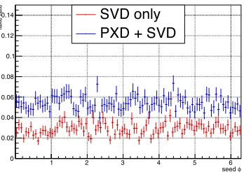
The results are summarized in Fig 5, the efficiency abovept∼50 MeV/c exceeds 80%. The fake

rate, before the final Kalman filter selection, is foreseen to be 0.06%. Figure 6 shows the fake rate as a function of the azimuth angleφ.

(GeV) t p 0.2 0.4 0.6 0.8 1 1.2 1.4 1.6

finding efficiency

0 0.2 0.4 0.6 0.8 1

SVD only PXD + SVD

(GeV) t p

0 0.05 0.1 0.15 0.2

finding efficiency

0 0.2 0.4 0.6 0.8 1

SVD only PXD + SVD

Figure 5: Track finding efficiency relative to an ideal track finder as a function of the transverse momentum using only the hits detected by the SVD and using all the informations coming from the VXD (PXD+SVD). On the left-hand side the results for the efficiency are shown in the range from pt =0 GeV/c to pt =1.75 GeV/c. On the right-hand side the same results are shown in the range

frompt=0 GeV/c topt=200 MeV/c.

φ seed

1 2 3 4 5 6

fake rate

0 0.02 0.04 0.06 0.08 0.1 0.12

0.14 SVD only

PXD + SVD

Figure 6: Fraction of fake tracks (random combination of hits) found by the track finding algorithm as a function of the azimuth angleφusing only the hits detected by the SVD and using all the infor-mations coming from the VXD (PXD+SVD).

The code was extensively tested on a real working system during a test beam in DESY in which a slice of the whole VXD system ( i.e. 2 PXD and 4 SVD ladders ) was read out by a scaled version the Belle II DAQ and HLT system. The code was able to sustain a trigger rate of a few kHz and to produce ROI for the PXD.

The start of the Beast II data taking is foreseen in late February 2018, time by which the parameters of the algorithms will be fully tuned.

References

[1] J. Lettenbichler, Ph.D. thesis, Technische Universität Wien (2016) [2] T. Bilka et al., IEEE Trans. Nucl. Sci.62, 1155 (2015),1406.4955 [3] T. Abe et al. (Belle-II) (2010),1011.0352

[4] H.G. Moser (DEPFET), Nucl. Instrum. Meth.A831, 85 (2016) [5] D. Dutta et al., JINST12, C02074 (2017)

[6] T. Schlüter (Belle-II Software Group), PoSVertex2014, 039 (2014),1411.3485

[7] A. Glazov, I. Kisel, E. Konotopskaya, G. Ososkov, Nucl. Instrum. Meth.A329, 262 (1993) [8] A. Strandlie, R. Fruhwirth, Nucl. Instrum. Meth.A480, 734 (2002)