Spatial and Temporal Risk Assessment for Water Resources Decision Making

(1)

Western University Western University

Scholarship@Western

Electronic Thesis and Dissertation Repository

9-15-2010 12:00 AM

Spatial and Temporal Risk Assessment for Water Resources

Decision Making

Shohan S. Ahmad

University of Western Ontario Supervisor

Slobodan P. Simonovic

The University of Western Ontario

Graduate Program in Civil and Environmental Engineering

A thesis submitted in partial fulfillment of the requirements for the degree in Doctor of Philosophy

Follow this and additional works at: https://ir.lib.uwo.ca/etd

Recommended Citation Recommended Citation

Ahmad, Shohan S., "Spatial and Temporal Risk Assessment for Water Resources Decision Making" (2010). Electronic Thesis and Dissertation Repository. 20.

https://ir.lib.uwo.ca/etd/20

This Dissertation/Thesis is brought to you for free and open access by Scholarship@Western. It has been accepted for inclusion in Electronic Thesis and Dissertation Repository by an authorized administrator of

(2)

SPATIAL AND TEMPORAL RISK ASSESSMENT FOR

WATER RESOURCES DECISION MAKING

(Spine title: Spatial & Temporal Water Resources Risk Assessment)

(Thesis format: Monograph)

By

Shohan S. Ahmad

Graduate Program in Engineering Sciences Department of Civil and Environmental Engineering

A thesis submitted in partial fulfillment of the requirements for the degree of

Doctor of Philosophy

The School of Graduate and Postdoctoral Studies The University of Western Ontario

London, Ontario, Canada

(3)

THE UNIVERSITY OF WESTERN ONTARIO

FACULTY OF GRADUATE STUDIES

CERTIFICATE OF EXAMINATION

Supervisor Examining Board

Dr. Slobodan P. Simonovic Dr. Raouf E. Baddour

Dr. Craig Miller

Dr. Micha Pazner

Dr. Niru Nirupama

The Thesis by

Shohan S. Ahmad

entitled:

SPATIAL AND TEMPORAL RISK ASSESSMENT

FOR WATER RESOURCES DECISION MAKING

is accepted in partial fulfillment of the

Requirements for the degree of

Doctor of Philosophy

Date : 15th September 2010 Lisa Hodgetts

(4)

ABSTRACT

Water resources systems are vulnerable to natural disasters such as floods, wind storms,

earthquakes, and various meteorological events. Flooding is the most frequent natural

hazard that can cause damage to human life and property. A new methodology presented

in this thesis is capable of flood risk management by: (a) addressing various uncertainties

caused by variability and ambiguity; (b) integrating objective and subjective flood risk;

and (c) assisting the flood risk management based on better understanding of spatial and

temporal variability of risk. The new methodology is based on the use of fuzzy reliability

theory. A new definition of risk is used and described using three performance indices (i)

a combined fuzzy reliability-vulnerability, (ii) fuzzy robustness and (iii) fuzzy resiliency.

The traditional flood risk management relies on either temporal or spatial variability, but

not both. However, there is a need to understand the dynamic characteristics of flood risk

and its spatial variability. The two-dimensional (2-D) fuzzy set that relates the universe of

discourse and its membership degree, is not sufficient to address both, spatial and

temporal, variations of flood risk. The theoretical contribution of this study is based on

the development of a three dimensional (3-D) fuzzy set.

The spatial and temporal variability of fuzzy performance indices – (i) combined

reliability-vulnerability, (ii) robustness, and (iii) resiliency – have been implemented to

(i) river flood risk analysis and (ii) urban flood risk analysis. The river flood risk analysis

is illustrated using the Red River flood of 1997 (Manitoba, Canada) as a case study. The

urban flood risk analysis is illustrated using the residential community of Cedar Hollow

(5)

The final results of the fuzzy flood reliability analysis are presented using maps that show

the spatial and temporal variation of reliability-vulnerability, robustness and resiliency

indices. Maps of fuzzy reliability indices provide additional decision support for (a) land

use planning, (b) selection of appropriate flood mitigation strategies, (c) planning

emergency management measures, (d) selecting an appropriate construction technology

for flood prone areas, and (e) flood insurance.

Key Words: Water resources, flood risk analysis, flood management, uncertainty

analysis, fuzzy sets, spatial and temporal fuzzy performance indices, floodplain mapping,

(6)

DEDICATION

I dedicate this thesis to my wonderful wife, Twiggy and my baby girl, Ereen who make

(7)

ACKNOWLEDGEMENTS

I wish to express my deepest appreciation to Professor Slobodan P. Simonovic, the

person that made all this research possible. He has provided an exceptional level of

guidance and supervision throughout the years, and for that I am most grateful. His

invaluable guidance and inspiration helped me grow confidence and develop both

academically and personally. Thank you very much Professor.

I would like to thank the Department of Civil and Environmental Engineering at the

University of Western Ontario, including faculty, staff, friends in the FIDS office, and

fellow graduate students. Away from school my wife, Twiggy reminded me that there is

life outside school, and kept me healthy and happy. Without her encouragement and

support, this achievement could not have been possible. I would like to thank my parents,

Dr. Sohrabuddin Ahmad and Mrs. Chaman Ara Ahmad; and Twiggy’s parents, Dr. Md.

Nurul Islam and Mrs. Saki Nazrin, who have always been a great encouragement for this

great achievement. Special thanks to Taufiq and Tansu.

Finally, I am grateful to the Natural Sciences and Engineering Research Council

(NSERC) of Canada for their very generous scholarships, which funded me throughout

my time in Civil and Environmental Engineering at the University of Western Ontario.

(8)

LIST OF FIGURES

FIGURE 1.1: GREAT NATURAL DISASTERS 1950-2009, NUMBER OF EVENTS (AFTER

MUNICH RE, NATCATSERVICE, 2010) ... 2

FIGURE 1.2: GREAT NATURAL DISASTERS 1950-2009, OVERALL AND INSURED LOSSES (AFTER MUNICH RE, NATCATSERVICE, 2010) ... 2

FIGURE 1.3: GREAT NATURAL DISASTERS 1950-2009, PERCENTAGE DISTRIBUTION (AFTER MUNICH RE, NATCATSERVICE, 2010) ... 3

FIGURE 1.4: SCHEMATIC OF CHAPTER 3... 10

FIGURE 2.1: MAJOR SOUCES OF UNCERTAINTY (AFTER SIMONOVIC, 1997) ... 15

FIGURE 2.2: DEFINITION OF PROBABILISTIC RISK (AFTER GANOULIS 1994) ... 29

FIGURE 2.3: DIFFERENT PERCEPTION OF FAILURE (AFTER EL-BAROUDY AND SIMONOVIC, 2004) ... 38

FIGURE 2.4: FUZZY REPRESENTATION OF ACCEPTABLE FAILURE REGION (AFTER EL-BAROUDY AND SIMONOVIC, 2004) ... 39

FIGURE 2.5: TRIANGULAR SYSTEM-STATE MEMBERSHIP FUNCTION ... 42

FIGURE 2.6: TWO COMPLIANCE CASES (EL-BAROUDY AND SIMONOVIC, 2004) ... 43

FIGURE 2.7: COMPATIBILITY WITH DIFFERENT LEVELS OF PERFORMANCE MEMBERSHIP FUNCTIONS (EL-BAROUDY AND SIMONOVIC, 2004)... 45

FIGURE 2.8: FUZZY REPRESENTATION OF MAXIMUM RECOVERY TIME ... 47

FIGURE 3.1: SCHEMATIC OF (I) RIVER, AND (II) URBAN FLOOD RISK ANALYSIS... 50

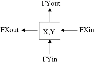
FIGURE 3.2: SINGLE CELL WITH INFLOW AND OUTFLOW. ... 58

FIGURE 3.3: GRAPHICAL RELATIONSHIP OF PERCENTAGE OF AVERAGE YIELD AND SEEDING DATE... 60

FIGURE 3.4: DEPTH-DAMAGE RELATIONSHIP FOR A RING DIKED COMMUNITIES... 63

FIGURE 3.5: 2-D FUZZY REPRESENTATION OF SPATIAL VARIABILITY IN ACCEPTANCE LEVEL OF PARTIAL FLOOD DAMAGE (AHMAD AND SIMONOVIC, 2007) ... 68

FIGURE 3.6: 3-D FUZZY REPRESENTATION OF SPATIAL AND TEMPORAL VARIABILITY IN ACCEPTANCE LEVEL OF PARTIAL FLOOD DAMAGE ... 68

FIGURE 3.7: 2-D FUZZY SET FOR TEMPORAL VARIABILITY OF FLOOD DAMAGE... 72

FIGURE 3.8: 2-D FUZZY SET FOR SPATIAL VARIABILITY OF FLOOD DAMAGE... 74

FIGURE 3.9: 3-D JOINT FUZZY SET OF FLOOD DAMAGE ... 75

FIGURE 3.10: CENTER OF GRAVITY OF THE 2-D FUZZY SET FOR TEMPORAL VARIABILITY... 77

FIGURE 3.11: 2-D FUZZY SET FOR SPATIAL VARIABILITY OF FLOOD DAMAGE AT G i D ... 78

(13)

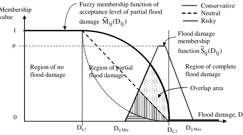
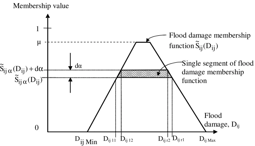
FIGURE 3.13: OVERLAP AREA BETWEEN FLOOD DAMAGE MEMBERSHIP FUNCTION AND

ACCEPTANCE LEVEL OF PARTIAL FLOOD DAMAGE MEMBERSHIP FUNCTION... 81

FIGURE 3.14: WEIGHTED AREA CALCULATION FOR THE FLOOD DAMAGE MEMBERSHIP FUNCTION ... 83

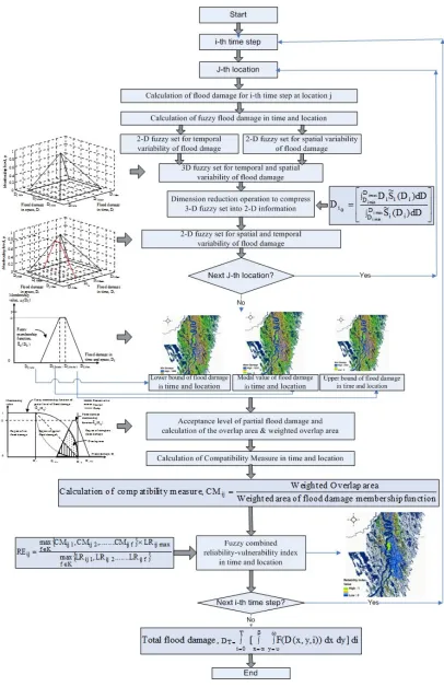
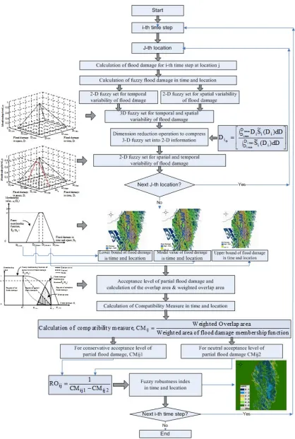
FIGURE 3.15: FLOW CHART OF FUZZY COMBINED RELIABILITY-VULNERABILITY INDEX 88 FIGURE 3.16: FLOW CHART OF FUZZY ROBUSTNESS INDEX ... 90

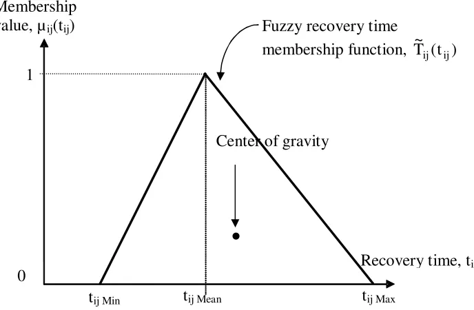
FIGURE 3.17: FUZZY MEMBERSHIP FUNCTION OF RECOVERY TIME ... 94

FIGURE 3.18: LAYOUT OF PIPE AND STREET SYSTEM (AFTER MARK ET AL., 2004)... 98

FIGURE 3.19: FLOW FROM THE STREET SYSTEM INTO A PARTLY FULL PIPE (AFTER MARK ET AL.,2004)... 98

FIGURE 3.20: FLOW TO THE STREETS FROM A PIPE SYSTEM WITH INSUFFICIENT CAPACITY (AFTER MARK ET AL., 2004) ... 99

FIGURE 4.1: CANADIAN PORTION OF THE RED RIVER BASIN (AFTER WINNIPEG FREE PRESS)... 125

FIGURE 4.2: SCHEMATIC DIAGRAM OF THE FLOOD CONTROL STRUCTURES... 129

FIGURE 4.3: SCHEMATIC DIAGRAM OF THE INFRASTRUCTURE IN THE STUDY AREA... 130

FIGURE 4.4: TOPOGRAPHIC DATA OF THE RED RIVER CASE STUDY ... 132

FIGURE 4.5: SCHEMATIC DIAGRAM OF 2-D MODELING APPROACH... 133

FIGURE 4.6: GUI WITH PREDEFINED PARTIAL LEVEL OF FLOOD DAMAGE FOR RED RIVER FLOOD 1997 ... 135

FIGURE 4.7: WATER SURFACE ELEVATION (M) IN RED RIVER FLOOD IN 1997... 137

FIGURE 4.8: SATELLITE IMAGE (LEFT) AND SIMULATED FLOODED AREA (RIGHT) ON MAY 1, 1997... 138

FIGURE 4.9: COMPARISON OF OBSERVED AND SIMULATED WATER ELEVATIONS (IN METER) AT RED RIVER NEAR ST ADOLPHE ... 139

FIGURE 4.10: COMPARISON OF OBSERVED AND SIMULATED WATER LEVELS AT FLOODWAY INLET... 139

FIGURE 4.11: SPATIAL AND TEMPORAL VARIATION OF FLOOD DAMAGE ($ PER 625 SQ. METER) ... 142

FIGURE 4.12: FUZZY COMBINED RELIABILITY-VULNERABILITY INDEX ... 145

FIGURE 4.13: SENSITIVITY ANALYSIS ON COMBINED RELIABILITY-VULNERABILITY INDEX TO THE SHAPE ... 149

FIGURE 4.14: FUZZY ROBUSTNESS INDEX ... 151

FIGURE 4.15: FUZZY RESILIENCY INDEX... 155

FIGURE 4.16: TOPOGRAPHIC DATA OF THE RED RIVER CASE STUDY ... 156

FIGURE 4.17: STUDY AREA DIVIDED INTO CELLS. ... 159

(14)

FIGURE 4.19: CONTROL SCREEN OF THE RED RIVER SECTION SIMULATION MODEL. ... 163

FIGURE 4.20: GUI WITH PREDEFINED PARTIAL LEVEL OF FLOOD DAMAGE ... 164

FIGURE 4.21: SPATIAL AND TEMPORAL VARIATION OF FLOOD DAMAGE ($ PER 4 SQ. KM) ... 165

FIGURE 4.24: FUZZY RESILIENCY INDEX... 171

FIGURE 4.25: LOCATION OF CEDAR HOLLOW, LONDON, ON... 172

FIGURE 4.26: 500 YEAR 6-HOUR DESIGN RAINFALL ... 175

FIGURE 4.27: FIA BASED STRUCTURE DEPTH-DAMAGE CURVE, TWO OR MORE STORIES WITH BASEMENT (SCAWTHORN, 2006)... 176

FIGURE 4.28: ROAD BLOCKAGE VS. PERCENT DAMAGE RELATIONSHIP ... 177

FIGURE 4.29: GUI WITH PREDEFINED PARTIAL LEVEL OF FLOOD DAMAGE FOR CEDAR HOLLOW... 178

FIGURE 4.30: SPATIAL AND TEMPORAL VARIATION OF WATER SURFACE ELEVATION (METER)... 180

FIGURE 4.31: SPATIAL AND TEMPORAL VARIATION OF DIRECT DAMAGE ... 182

FIGURE 4.32: SPATIAL AND TEMPORAL VARIATION OF INDIRECT DAMAGE ... 183

FIGURE 4.33: SPATIAL AND TEMPORAL VARIATION OF TOTAL FLOOD DAMAGE ... 184

LIST OF TABLES

TABLE 4.1: COMPARISON OF RECORDED AND MODELED PEAK WATER LEVELS (FT) FOR 1997... 140

TABLE 4.2: AREA IN SQUARE KM CORRESPONDING TO VALUES OF COMBINED RELIABILITY-VULNERABILITY INDEX ... 148

(15)

1 INTRODUCTION

1.1 WATER RESOURCES MANAGEMENT UNDER UNCERTAINTY

Uncertainty can have important implications on water resources management. All water

management decisions should take uncertainty into account. The diversity of sources of

uncertainty in water resources management pose a great challenge to ensure a satisfactory

and reliable system performance. Sometimes the implications of uncertainty are the risks

associated with the potential and significant effects of poor water resources system

performance. Adopting high safety factors by considering all unknown sources of risk

(standard-based engineering practice) is one of the ways to avoid uncertainty. However, a

high safety factor without quantifying different sources of uncertainty would make the

solution infeasible. Therefore it is necessary to quantify known sources of uncertainty.

Managers need to understand the nature of the underlying threats in order to identify,

assess and manage the risks associated with uncertainty. The inability to do so is likely to

result in adverse impacts on systems performance, and in extreme cases such as natural

hazards, i.e. floods, cyclones, tsunamis etc, this can result in catastrophic performance

failures. Quantification of uncertainty in natural hazard risk management can reduce the

loss of lives and damage to properties. According to Simonovic (2011) the longer time

period records (traced back to 1900 while more reliable after 1950) show an increasing

trend in the number of disasters (Figure 1.1), their overall and insured losses (Figure 1.2),

(16)

Figure 1.1: Great natural disasters 1950-2009, number of events (after Munich Re,

NatCatService, 2010)

Figure 1.2: Great natural disasters 1950-2009, Overall and insured losses (after Munich

(17)

Figure 1.3: Great natural disasters 1950-2009, percentage distribution (after Munich Re,

NatCatService, 2010)

In 2000, Mozambique was affected by a devastating flood that made half a million people

homeless and caused 700 deaths (Wheater, 2005). The devastating flood of Central

Europe in 2002 required the widespread evacuation of many towns and cities, with

property damage estimated at 21.5 billion euros (Kron, 2005; Wheater, 2010). On July

26, 2005, the flooding that took place in Mumbai (Bombay) affected approximately 5

million people and led to 1000 deaths. 940 millimeters of rainfall was recorded in this

single event. Flooding in Central Europe in August 2005 caused fatalities in Germany,

Switzerland, Austria, Romania and Bulgaria (Wheater, 2010). Among recent incidents, a

flood of southern China in June 2010 affected more than 29 million people and inundated

1.6 million hectares of agricultural land. More than two million people were evacuated

and 195,000 houses collapsed, with direct economic losses amounting to approximately

(18)

Central Europe affected Austria, the Czech Republic, Germany, Hungary, Poland,

Slovakia, Serbia and Ukraine. Poland was the worst affected and the city of Kraków

declared a state of emergency. As a result of the devastating flood 37 people were killed

and approximately 23,000 people were evacuated. Poland estimated an economic loss of

2.5 billion euros (Euronews, 2010).

Urban flooding also poses a major threat to many cities around the world. Higher

frequency of urban flooding, which occurs mostly in developing countries, has made it

necessary for the development of a more efficient urban flood management plan. Heavy

rainfall, combined with an insufficient capacity of sewer systems, can cause urban

flooding. In February 2002, 50 people were killed and 200,000 people made homeless in

Indonesia as a result of heavy rainfall that led to urban flooding (Mark et al., 2004). In

2000, Mumbai experienced a major flooding event in which 15 lives were lost and that

caused immeasurable inconveniences for many people living in that region. In Dhaka

City (Bangladesh), due to an insufficient capacity of storm sewer systems, a small rainfall

event can cause serious problems. In September 1996, Dhaka City was paralyzed as a

result of urban flooding. In 1983, Bangkok (Thailand) remained flooded for almost 6

months and reported infrastructure damage was approximately $146 million (Mark et al.,

2004). On August 19, 2005, a two to three hour period of extremely heavy rainfall hit the

Greater Toronto Area and quickly caused an accumulation of storm water in the storm

sewer systems, which resulted in flooding across the city. This single rain event cost the

city an estimated $34 million. In addition, the Insurance Bureau of Canada estimated that

(19)

caused by this single storm event (River Sides, 2005). Toronto was not alone in

experiencing first hand the destructive potential of flooding. In February 2010, heavy rain

lashed the Portuguese resort island of Madeira, turning some streets in the capital,

Funchal, into raging rivers of mud, water and debris. The mudslides and flooding killed

at least 42 people and more than 120 other people were reported as injured (CBC news,

2010). In April, 2010, landslides and floods set off by the heavy rains killed at least 95

people in the city of Rio de Janeiro. In addition to obstructing roads and other

infrastructure, the devastation caused by this flood resulted in hundreds of people

becoming homeless, virtually paralyzing the economic activity of Brazil’s second largest

city (Reuters, 2010).

Ganoulis (1994) argues that engineering risk assessment and reliability analyses provide

a general methodology for the quantification of uncertainty and, as a result, should be

used to determine the safety of an engineering system. Risk assessment is an essential

component of sustainable flood management, and is becoming more important with the

increase in population density and the intensifying effects of climate change. There is a

scientific consensus that climate change is resulting in higher average temperatures,

rising sea levels, change in precipitation patterns and change in frequency and severity of

extreme hydrological conditions – floods and droughts. A larger population affects the

sustainability of land use, safe economic development in flood prone areas, and in

general leads to greater flood vulnerability.

(20)

floods: (a) structural measures; and (b) non-structural measures (Simonovic, 1999 among

others). The most common structural interventions used today are: (i) levees or flood

walls; (ii) diversion structures; (iii) channel modifications; and (iv) flood control

reservoirs. For management of urban floods, the structural measures now deal with

efficient storm sewer system and infiltration basin. Furthermore, the structural measures

are becoming more frequently combined with non-structural measures, such as flood

zoning, flood warning, waterproofing, and flood insurance. Levy and Hall (2005)

introduced the important concept of “living with flood”, which requires a high public

awareness of actual flood risks. The quantification of all uncertainties and the spatial and

temporal representation of flood risk contributes to a higher level of awareness and may

reduce the effects of flood damage to both people and material.

1.2 OBJECTIVE AND SUBJECTIVE UNCERTAINTY

There are many types of uncertainty in the flood management process, ranging from

hydrologic, hydraulic, geotechnical, and structural uncertainty, to economic,

environmental, ecological, social and political uncertainty. According to Slovic (2000)

and Simonovic (2002) a major part of the confusion implicit in flood risk analysis relates

to an inadequate distinction between three fundamental concepts of probability and risk:

(i) Objective risk (real, physical), Ro, and objective probability, po, which is the property

of real physical systems; (ii) Subjective risk, Rs, and subjective probability, ps; and (iii)

Perceived risk, Rp, which is related to an individual’s feeling of fear in the face of an

undesirable and possible event. Probability is here defined as the degree of belief in a

(21)

may be some function of Ro and po). Similarly, Rp is not a property of the physical

systems but is related to fear of the unknown. Moreover, Rp may be a function of Ro, po,

Rs, and ps . Because of the confusion between the concepts of objective and subjective

flood risk, many characteristics of subjective risk are also believed to be valid for

objective risk. Indeed, it is almost universally assumed that the imprecision of human

judgment is equally prominent and destructive for all water resources risk evaluations and

all risk assessments. The popular methods used by society to manage flood risk appear to

be dominated by considerations of perceived and subjective risks, while it is the objective

risks that kill people, damage the environment and create property loss (Simonovic and

Ahmad, 2007).

1.3 SPATIAL AND TEMPORAL CHARACTERISTICS OF FLOOD RISK

Flood risk assessments have three main characteristics: (i) spatial structure and

relationships among risk characteristics; (ii) interactions among the spatial risk

characteristics; and (iii) changes or alterations in temporal risk characteristics. Any effort

to understand and describe the dynamics of flood risk assessment requires the ability to

deal with these interrelated aspects. Traditional modeling approaches focus on either

temporal or spatial variation, but not both. There is an important feedback between time

and location in space, i.e., temporal variability of risk is affected by the change of spatial

characteristics of risk. To understand risk dynamics, patterns in time and location in

space need to be examined together. Therefore, to better understand dynamic

characteristics of flood risk, a new modeling framework is required that not only captures

(22)

tools required for solving complex flood risk management problems. Modeling

environments that can link social, economic, and environmental consequences of flood

risks are fundamental to an understanding of the impacts of proposed management

decisions. An integrated modeling framework can enhance our ability to understand

complex flood management processes, and can also assist in generating adequate

information/scenarios in order to help decision-making.

1.4 OBJECTIVES OF THE RESEARCH

The main objectives of the research presented here are (a) to provide the methodology for

flood risk assessment while taking into consideration the spatial and temporal variability

of various objective and subjective uncertainties in flood management, and (b) to provide

a methodology possessing the capability to spatially and temporally represent integrated

flood risk. The presented research develops three fuzzy performance indices: (1)

combined reliability-vulnerability index, (2) robustness index, and (3) resiliency index,

for spatial and temporal reliability analysis of riverine and urban floods. This new

methodology is not limited by the shape of the membership function in any way. The

shape of the membership function that best represents the flood damage should be

selected on the basis of the available damage information and the stakeholder’s domain

knowledge. The existing literature offers various methods for the development of

appropriate membership functions that combine data, expert opinion and stakeholder’s

preferences. Despic and Simonovic (2000) provide a methodology for developing an

appropriate membership function for flooding. Since the main focus of this thesis is on

(23)

a triangular fuzzy membership function is used for the purposes of illustration. Sensitivity

analyses are also performed using a trapezoidal membership function to emphasize the

importance on choosing the right membership function.

1.5 RESEARCH CONTRIBUTIONS

The traditional two-dimensional (2-D) fuzzy set representation is not sufficient to handle

both spatial and temporal information. The theoretical foundation of this study is based

on the development of a three dimensional (3-D) fuzzy set representation of the flood risk

that includes spatial and temporal variability. In order to describe the spatial and temporal

variability in the risk preferences of decision makers, the proposed methodology extends

the partial flood damage concept (El-Baroudy and Simonovic, 2004) to a 3-D

representation. The practical contribution of this research is the development of a flood

risk management approach capable of:

addressing uncertainty caused by spatial and temporal variability and ambiguity;

integrating objective and subjective risks; and

assisting flood management decision making by providing a better understanding

of spatial and temporal variability of risk.

1.6 ORGANIZATION OF THE THESIS

This thesis contains five chapters. The first chapter is a general introduction to flood risk

assessment. The second chapter contains a literature review on water resources

management (mainly focusing on floodplain management) under uncertainty, modeling

(24)

performance indices developed by El-Baroudy and Simonovic (2004) that forms the basis

of the research presented in this thesis. The third chapter provides the methodology

adopted for the spatial and temporal extension of the fuzzy reliability analysis of flood

risk. The third chapter presents the mathematical formulation in two parts:

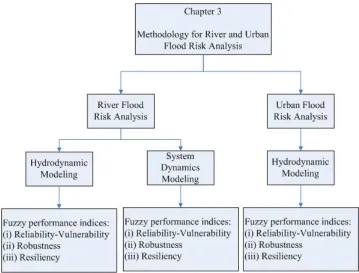
Figure 1.4: Schematic of Chapter 3

(a) the first part describes the methodology of spatial and temporal reliability analysis

for river flooding. The dynamic process of overland flooding is addressed using

two modeling tools: (i) hydrodynamic modeling, and (ii) system dynamics (SD)

modeling. The results of these two models are water surface elevations for

different time steps and locations in space. The presented methodology then uses

(25)

damage, and develops the fuzzy performance indices to spatially and temporally

represent reliability-vulnerability, robustness and resiliency for river flood risk.

(b) the second part describes the methodology used for the spatial and temporal

reliability analysis for urban flooding. The dynamic interaction between the storm

sewer network and overland flow is addressed using a hydrodynamic modeling

tool. Due to the inadequate capability of the SD approach to dynamically link a

storm sewer model with an overland flow model, SD modeling is inappropriate to

address overland flooding for an urban flood context. As such, the hydrodynamic

modeling is used to simulate the dynamic process of overland urban flooding. The

hydrodynamic model generates water surface elevations for different time steps

and locations, which are used to determine the spatial and temporal variation of

flood damage. The methodology then develops the fuzzy performance indices to

spatially and temporally represent reliability-vulnerability, robustness and

resiliency of urban flood risk.

Chapter four demonstrates the applicability of the proposed approach for two case

studies: (i) Red River flood risk analysis, Manitoba, Canada, and (ii) Urban flood risk

analysis for London, Ontario, Canada. Finally, summaries and conclusions of the

(26)

2 LITERATURE REVIEW

Engineering risk and reliability analysis is a general methodology for the quantification

of uncertainty and the evaluation of its consequences for the safety of engineering

systems (Ganoulis, 1994). Risk identification is the first step in any risk analysis, where

all sources of uncertainty are clearly detailed. Quantification of risk is the second step,

where uncertainties are measured using different system performance indices and figures

of merit such as reliability, vulnerability, robustness and resiliency. The existence of

different types of uncertainty creates many challenges in water resources planning, design

and management. Therefore reliability analysis in water resources management relies

greatly on the proper quantification of different sources of uncertainty.

This chapter first introduces different types of uncertainty, i.e. inherent spatial and

temporal variability associated with water resources management. The chapter then

focuses on different modeling approaches to address the dynamic process of water

resources system (such as flood risk), and their spatial variability. The dynamic

characteristics of flood risk and its spatial variability are difficult to understand due to the

inherent complexity of human and natural systems. Traditional modeling approaches

focus on either temporal or spatial variation, but not both. There is a need to understand

the dynamic processes and their interaction in time and location in space. In case of water

resources systems, particularly for flood processes, different modeling tools are required

that capture dynamic processes in time and location in space. The dynamic process of

overland flooding is presented in this research using two modeling tools: (i)

(27)

reviews different approaches used in the framework of reliability analyses of engineering

systems. The chapter focuses on the fundamentals of the probabilistic reliability analysis.

This part focuses on the use of performance indices for evaluating risk and reliability in

water resources management. Since the probabilistic approach faces great challenges in

addressing uncertainty related to human subjectivity and ambiguity, this chapter sheds

light on the importance of subjective uncertainty in water resources management and

shows the capability of different methods to overcome the shortcomings and limitations

of probabilistic reliability analysis. Next, this chapter introduces the fuzzy set theory as a

complementary approach for assessing uncertainty related to water resources systems and

focuses on the use of fuzzy performance indices for reliability analysis.

2.1 WATER RESOURCES MANAGEMENT UNDER UNCERTAINTY

Tung and Yen (2005) define uncertainty as “the occurrence of uncontrollable events”.

Decisions in engineering-based systems design, planning, and management are made

with uncertainty, the sources of which are many and diverse. Ang and Tang (1984) point

out that there is uncertainty in all engineering-based systems because these systems rely

on the modeling of physical phenomena that are either inherently random or difficult to

model with a high degree of accuracy. All water management decisions should take

uncertainty into account. Implications of uncertainty may be risks in the sense of

significant potential unwelcome effects of water resources system performance.

Accordingly, if analysis of the performance of a water resources system does not

adequately consider different types and sources of uncertainty, the extent of damage

(28)

these in mind, managers need to understand the nature of the underlying threats in order

to identify, assess and manage risk. Failure to do so is likely to result in adverse impacts

on performance, and in extreme cases, major performance failures.

2.2 TYPES OF UNCERTAINTY

Different classifications of types and sources of uncertainty exist in the literature

depending on the considered aspect of uncertainty. For example, uncertainty in water

resources systems can be attributes to hydrologic, structural, environmental, social,

economical, and operational aspects. Tung and Yen (2005) list some of those

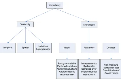
classifications. According to Simonovic (1997) and NRC (2000) the taxonomy of

uncertainty includes: (1) natural variability and (2) knowledge uncertainty (Figure 2.1).

Natural variability deals with variability inherent to the physical world, viz. events that

can be described as “random”. Simonovic (1997) further categorized natural variability,

i.e. randomness, into i) temporal variability, ii) spatial variability, and iii) individual

heterogeneity. Temporal variability describes the time dependent fluctuations, while

spatial variability describes the space dependent fluctuations. In this thesis spatial

variability refers to location dependent fluctuations. Individual heterogeneity includes all

other sources of variability. The second type of uncertainty, knowledge uncertainty, deals

with a lack of understanding of events or processes. According to Simonovic (1997),

knowledge uncertainty reflects our limited ability to represent real world phenomena

with a mathematical model for effective analysis, which can have an effect on i) model

formulation, ii) parameter estimation, and iii) decision-making. Knowledge uncertainty

(29)

processes (NRC, 2000).

Figure 2.1: Major souces of uncertainty (after Simonovic, 1997)

In flood risk management variability is mainly associated with the spatial and temporal

variation of the main hydrologic variables (precipitation, river flow, etc). The temporal

variability of flow results in variations of flood water level. The shape of the hydrograph

can have a significant impact on the extent of flood damage. Depending on the rainfall

intensity, rainfall duration, and the direction of storm movement, there can be a wide

range of hydrograph shapes. Spatial and temporal variability of these factors may

augment or reduce peak flow, cause either a gradual or rapid rise to peak value, and also

result in gradual or rapid recession of the hydrograph. Gradual recession of the

(30)

to agricultural crops, infrastructure and property. In flood risk management spatial

variability is also associated with floodplain characteristics such as land-use, terrain

elevation, channel network, vegetation, roughness, soil characteristics, porosity, etc. For

example, areas closer to the river and with a lower elevation are highly prone to

significant flood damage compared to areas further away from the river with higher

elevations. As floods recede, areas with higher elevation are more quickly dried and are

ready to seed before areas closer to the river and with lower elevations. Uncertainty in

spatial and temporal variability arises due to our inability to accurately measure, calculate

or estimate the value of such factors.

In flood risk management, the uncertainty pertaining to the physical characteristics of the

water resources system is partly about variability. Uncertainty is, in part, also about lack

of knowledge or ambiguity. Both variability and ambiguity are associated with a lack of

clarity, which arises because of the typical lack of system performance history and

records, human error, subjectivity, faulty assumptions, bias and ignorance.

2.3 MODELING DYNAMIC PROCESS OF RIVER AND URBAN FLOODING

Risk in water resources management requires the understanding of three main

characteristics: (i) spatial structure and the relationships among risk characteristics; (ii)

interactions among the spatial risk characteristics; and (iii) changes or alterations in risk

characteristics over time (Simonovic, 2007). In order to deal with the dynamic

characteristics of flood, it is essential to understand and describe all of its interrelated

(31)

characteristics of flood risk have not been fully considered in traditional modeling

approaches. Normally such approaches focus on either temporal or spatial variation, but

not both. There is a need to understand the important interactions between time and

location in space, i.e., how the temporal variability of risk is affected by a change in the

spatial characteristics of risk. Therefore in order to properly address risk dynamics, the

spatial and temporal characteristics of risk need to be examined together. The work

presented in this thesis focuses on the development of a new modeling framework that

not only captures dynamic processes in time and location in space but also integrates

different modeling tools required for solving complex river and urban flood management

problems. Ahmad and Simonovic (2004) introduced three modeling paradigms: (i)

cellular automata (CA), (ii) geographic information system (GIS), and (iii) system

dynamics (SD), which exhibit the potential for describing dynamic processes in time and

location in space. In this research, system dynamics (SD) is presented as a strong

modeling tool for modeling the spatial and temporal characteristics of overland flooding.

This research also introduces hydrodynamic modeling as another strong tool capable of

modeling the dynamic interactions on the propagation of river and urban flooding, and

also for addressing the spatial and temporal variability of overland flow. The following

sections provide a brief description of the strengths, weaknesses and applicability of these

two modeling approaches - (i) hydrodynamic modeling, and (ii) system dynamics

modeling – for addressing overland flooding in flood risk management.

2.3.1 HYDRODYNAMIC MODELING

(32)

water depth, velocity, and the extent of inundation of a flooding event, all of which are

very important in flood risk analysis. Flows for which flood water depth and velocity

vary, not only with location in space but also with time, are considered as transient or

unsteady flow. In rivers and floodplains, flows can be considered as steady for the

purposes of an approximate representation of overland flooding in time and location in

space. However, for more accurate modeling, the analysis of overland flooding requires

considering the flow as unsteady or transient. In 1871, Barrède Saint-Venant formulated

the basic theory that considered the analysis of unsteady flow through the coupling of the

continuity and momentum equations. Modeling of fluid flow is possible either as

one-dimensional, where the direction of flow is predetermined and thereby making

approximation or as two-dimensional, where the direction of flow is not predetermined,

and is therefore not restricted.

The hydrodynamic modeling used in this research is presented as a powerful tool for

addressing river and urban flooding and also for modeling spatial and temporal variability

in flood water level, discharge, velocity, etc. Flow in rivers and through pipes can be

accurately modeled considering one-dimensional representation. However, consideration

of one-dimensional representation will not accurately model overland flooding. Therefore

the flow should be considered as unsteady or transient while modeling overland flooding

in two-dimensions. Since an analytical solution of the Saint-Venant equations is not

possible, the complete Saint-Venant equations must be solved numerically for overland

flooding. The most common numerical solutions to the Saint-Venant equations are the

(33)

There are a number of studies that compare one-dimensional (1-D) and two-dimensional

(2-D) approaches in river flood modeling (Horritt and Bates, 2002; Lin et. al., 2006). In

confined channels, such as pipe networks, the 1D sewer model can provide acceptable

results as long as the water is contained within the street network (Mark et. al., 2004). If

the water overflows the curbs and flows overland, the flow may change direction. Under

these circumstances the 1D model should not be used, and the 2D model becomes the

preferred choice. Leandro, et al. (2009) also concluded that 1D models can provide an

adequate approximation of flow in confined channels (such as rivers, pipes and streets),

however 2D models give better results for the flow over terrain. Early urban hydrologic

models did not have the capability to model the excess flow from the manholes as

overland flooding. The surcharged flow remained atop of the manholes until the capacity

of the sewer networks was at a maximum. When sewer network capacity became

available, the excess water was allowed to drain back into the storm sewer network

(Rossman, 2005; Zhong, 1998). This shortcoming in the earlier storm sewer models was

overcome by introducing links between surface networks and pipe networks (Leandro et

al., 2009).

The use of hydrodynamic modeling in river and urban flooding is becoming very

common as the result of: (i) the time needed for the numerical modeling of full Saint

Venant equations has become more acceptable, (ii) an increased availability of high

resolution topographic data, such as LIDAR, which is required as input into the 2D

hydrodynamic model, and (iii) the accumulation of more detailed and accurate results of

(34)

investigation (Smith, et. al., 2006).

Some examples of the commercial tools used for 1D river modeling are HEC-RAS

(Hydraulic Engineering Center, 2010), MIKE 11 (DHI, 2008,(a)) and SOBEK (WL|Delft

Hydraulics, 2005). For 1D pipe flow modeling, examples include MOUSE (DHI, 2004),

MIKE URBAN (DHI, 2009), XP-SWMM (XP Software, 2010), EPA SWMM (EPA,

1995) and PC-SWMM (CHI, 2006). For 2D overland flow modeling examples include

MIKE 21 (DHI, 2008,(b)), TUFLOW (Phillips et. al., 2005), SOBEK, GSSHA (Charles

et. al., 2006), RMA2 (Barbara et. al., 2006). The commercial hydraulic/hydrodynamic

models, such as MIKE URBAN (DHI, 2009) or Infoworks CS (Wallingford Software,

2006) have the capability to model the dynamic interactions between surface networks

and pipe/sewer networks by using a weir or an orifice equation (Kawaike and Nakagawa,

2007; Mark et al., 2004; Nasello and Tucciarelli, 2005, Leandro et. al., 2007). Recently

there has been a growing trend towards integrating two or more hydrodynamic models to

overcome the weakness in linkage between two models. Examples of such models are

(1D/2D) MOUSE-MIKE21, which couples the 1D MOUSE pipe/sewer model with the

2D MIKE21 overland model (Carr and Smith, 2006); the (1D/2D) SOBEK Urban, which

couples the 1D SOBEK flow with 2D Delft FLS (Bolle et al., 2006); or TUFLOW. The

current trend in river flood modeling is to couple a 1D river model with a 2D

overland/surface flow model, and in the case of urban flood modeling, a 1D pipe flow

model is coupled with a 2D overland flow model. In certain cases all of the three models

– (i) 1D river model, (ii) pipe flow model, and (iii) overland flow model – may be

(35)

models (Kaushik, 2006; Chen et al., 2007). More recently, Leandro, et. al. (2009)

provided a comparison between a 1D sewer model coupled with a 1D surface network

model (1D/1D) and a 1D sewer model coupled with a 2D overland/surface flow model

(1D/2D).

There are certain limitations in 2D hydrodynamic modeling, such as computation time,

requirement of more data, etc. The computation time in 2D modeling is significantly

higher compared to 1D modeling (Paquier et al., 2003; Lhomme et al., 2006). However,

it should be noted that the 1D hydrodynamic model does not provide satisfactory results

for solving overland flow, in which case 2D hydrodynamic modeling is required.

2.3.2 SYSTEM DYNAMICS (SD) MODELING

System Dynamics (SD) is a rigorous method of system description, which facilitates

feedback analysis via a simulation model of the effects of alternative system structures

and the control policies of system behaviour (Simonovic, 2009). The advantages of

system dynamics simulation include: (a) facilitating the simplicity of use of system

dynamics applications; (b) a greater applicability of the general principles of system

dynamics to social, natural, and physical systems; (c) the ability to address how

structural changes in one part of a system might affect the behaviour of the system as a

whole; (d) a combined predictive (determining the behaviour of a system under

particular input conditions) and learning (the discovery of unexpected system behaviour

under particular input conditions) functionality; and (e) an active involvement of

(36)

largely in representing temporal processes. SD models, however, do not adequately

represent spatial processes. For example, SD models can be used for the analysis of

different flood management policies and the estimation of flood damages (as a function

of time). However, SD modeling provides no easy way to represent damage

topographically. A simple SD model is therefore inadequate for developing an overland

flood model that can capture both spatial and temporal variability in the propagation of

flood flows. Given that SD is adept at representing temporal processes (with a limited

capacity for spatial modeling), and GIS is useful for spatial modeling (with a limited

capacity for temporal representation), the logical step in the development of a more

comprehensive methodology is the integration of SD with GIS to model the

spatio-temporal dynamics of engineering systems.

System dynamics has a long history as a modeling paradigm with its origin in the work of

Forrester (1961), who developed the subject to provide an understanding of strategic

problems in complex dynamic systems. System dynamics is grounded in control theory

and the modern theory of nonlinear dynamics. More details on SD modeling can be found

elsewhere (Sterman, 2000; Ford, 1999; and Coyle, 1996). System Dynamics is a

promising approach for modeling complex dynamic systems. SD has been successfully

applied to policy analysis in the area of business (Sterman, 2000), health care (Royston et

al., 1999), and environmental management (Ford, 1999; and Sudhir et al., 1997). The

concepts and applications of system dynamics approaches to a variety of problems have

been discussed by several authors (Sterman, 2000; Forrester, 1961; and Coyle, 1996).

(37)

Palmer (1998) has done extensive work in river basin planning using SD. Keyes and

Palmer (1993b) used SD simulation modeling for drought studies. Matthias and Frederick

(1994) have used SD techniques to model sea-level rise in coastal areas. Fletcher (1998)

has used system dynamics as a decision support tool for the management of scarce water

resources. Simonovic, et. al., (1997) and Simonovic and Fahmy (1999) have used a SD

approach for long-term water resources planning and in policy analysis for the Nile River

Basin in Egypt. The SD approach has been used to model reservoir operation for flood

control (Ahmad and Simonovic, 2000a), operation of multiple reservoirs for hydropower

generation (Teegavarapu and Simonovic, 2000), calculation of flood damages (Ahmad

and Simonovic, 2000b), and analysis of the economic aspects of flood management

policies (Ahmad and Simonovic, 2000c). Simonovic (2002) has used SD to develop a

world water model. Li and Simonovic (2001) have developed a SD model for predicting

floods from snowmelt in North American prairie watersheds. Ahmad and Simonovic

(2001c) used SD as a decision support tool for the evaluation of impacts of flood

management policies. The spatial system dynamics approach (SSD) developed by Ahmad

and Simonovic (2004) can model dynamic processes in time and location in space with

certain limitations.

The strength of the system dynamics approach is in its ability to represent temporal

processes. SD models are excellent tools for planning and policy analysis. SD models,

however, do not adequately represent spatial processes. For example, system dynamics

models can be used for the analysis of different flood management policies and the

(38)

representing temporal processes with restricted spatial modeling capabilities, and the

competency of GIS for spatial modeling with limited representation of temporal aspects,

a logical alternative is the integration of system dynamics with GIS to model spatial

dynamic systems. Attempts have been made to add spatial dimensions to system

dynamics models. These attempts can be divided into two categories: (a) introducing

spatial dimensions into the system dynamics model (implicit approach) or (b) translating

system dynamics model equations to run in GIS. The first approach does not represent

spatial dimensions in an explicit manner. The Mono Lake model is an example of this

approach (Ford, 1999). In this model spatially important features of the system are

represented with one or two aggregate relationships. The complex shape of the Mono

basin affects the water flow, which is modeled by two non-linear functions: (a) surface

area – volume curve; and (b) elevation - volume curve. The second approach of adding a

spatial dimension to the system dynamics models involves translating SD model

equations into a programming language and interfacing with GIS. For instance, Costanza

et al. (1990) combined a GIS with a system dynamics model for ecological modeling.

They used Stella (HPS Inc., 2001) to develop ecological models and then translated the

model into Fortran through a separate program to interface with the GIS. To study the

effects of fire on landscape patterns Baker (1992) interfaced four models with a GIS to

control the simulation, data handling, and display. A decision support software package,

Extend and EML (Environmental Modeling Language), were used by Theobald and

Gross (1994) to explore landscape dynamics (a fire spread and population model). They

combined SD, GIS and CA to provide spatial-temporal modeling capabilities for

(39)

reported by Westervelt and Hopkins (1999) using software packages IMPORT/ DOME,

GRASS, and SME (Spatial Modeling Environment). In these studies, the work is focused

on spatial modeling (emphasis on GIS) and SD is used to bring the dynamic modeling

(temporal aspect) capability into the GIS environment. Since system dynamics model

equations are translated to run within a GIS, a drawback of the approach used in these

studies is the loss of the interactive power of SD (changes cannot be made during

simulation). The main limitation in all the attempts that have been made so far for a

combined spatio-temporal dynamic modeling, is that the relationship between time and

location in space is not explicit.

2.4 DEFINITION OF RISK

A standardized and overarching definition of risk is perhaps unachievable. Numerous

definitions can be found in the relevant literature as authors continue to define risk in

their own way. Simonovic (1997) defined risk as a measure of the probability and

severity of adverse effects. Simonovic and Ahmad (2007) further defined risk as the

“significant potential unwelcome effect of water resources system performance or the

predicted or expected likelihood that a set of circumstances over some time frame will

produce some harm that matters”. Haimes (1998) defines the risk analysis process as “a

set of logical, systematic and well-defined activities that provide the decision maker with

a sound identification, measurement, quantification, and evaluation of the risk associated

with certain natural phenomena or man made activities.” Normally, risk is equated with

the probability of failure or the probability of load exceeding resistance. Other symbolic

(40)

hazards divided by safeguards (Lowrance, 1976). According to Simonovic and Ahmad

(2007) there are three cautionary measures surrounding risk that must be taken into

consideration: (i) risk cannot be represented objectively by a single number alone, (ii)

risk cannot be quantified on strictly objective grounds, and (iii) risk should not be

labeled as real. Regarding the caution of viewing risk as a single number, the

multidimensional character of risk can only be aggregated into a single number by

assigning implicit or explicit weighting factors to various numerical measures of risk.

Since these weighting factors must rely on necessarily biased value judgments, the

resulting single metric for risk cannot therefore be deemed objective. Since risk cannot be

expressed objectively by a single number, it is not possible to rank risks on strictly

objective grounds. Finally, since risk estimates are evidence-based, risks cannot be

strictly labeled as real. Rather, they should be labeled as inferred, at best.

2.5 RISK IDENTIFICATION

Risk identification is the first step in any risk analysis, where all sources of uncertainty

are clearly detailed. Risk and reliability analysis can be used to assess the safety of any

engineering system (Ganoulis, 1994). Classical reliability analysis uses the

load-resistance approach (which is widely used in structural reliability analysis). Load, l, is a

variable that reflects the behaviour of the system under certain external conditions of

stress loading, while resistance, r, is a characteristic variable which describes the capacity

of the system to resist an external load. Failure occurs when the load exceeds the

resistance, while the system is considered safe if resistance exceeds or is equal to the load

(41)

FAILURE or INCIDENT : l > r

SAFETY or RELIABILITY : l ≤ r

The quantification of risk is the second step in any risk analysis, whereby uncertainties

are measured using different system performance indices such as reliability, vulnerability,

robustness and resiliency. Importantly, the quantification of uncertainties involved in

floodplain management can be used to mitigate the risks of flood damage.

2.6 PERFORMANCE INDICES

Performance Indices (PI) are measures of how well a system performs under various

loading conditions. Safety of the system under uncertainty can be represented by the

performance indices. Hashimoto et al. (1982a and 1982b) suggest reliability, resiliency,

vulnerability and robustness as performance indices to evaluate the performance of water

resources systems. Duckstein et al. (1987) mention incident-related performance indices

such as grade of service, quality of service, speed of response, incident period,

availability, economic index vector, in addition to the PIs suggested by Hashimoto et al.

(1982a and 1982b).

2.7 RELIABILITY ANALYSIS IN ENGINEERING SYSTEMS

Probability theory and fuzzy set theory are the main approaches used in the risk and

reliability analysis of engineering systems. The probabilistic approach and the fuzzy

(42)

2.7.1 PROBABILISTIC APPROACH IN WATER RESOURCES

MANAGEMENT

Analysis in the probabilistic approach involves describing load and resistance as

belonging to respective possible probability distributions. Uncertainty in both load and

resistance is introduced through the use of random variables. Therefore, the system

reliability is realistically measured in terms of probability. The principal objective of the

probabilistic reliability analysis is to ensure, in terms of probability, that load does not

exceed resistance throughout a specified time horizon in terms of probability.

Ganoulis (1994) states that by considering the system variables as random, uncertainties

can be quantified on a probabilistic framework. Load, l, and resistance, r, are taken as

random variables L and R, with the following probability distribution and probability

density distribution functions:

FL(l), fL(l) : load

FR(r), fR(r) : resistance

In the probabilistic framework, the simple definition of failure is when the load exceeds

the resistance. Thus probability of failure or risk is defined by the following relation:

PF = P(R<L) (2.1)

The quantity PF is obtained by the joint probability density function fLR(l,r) of the

random variables R and L. Figure 2.2 shows the risk PF above the bisectrice line L=R

(43)

PF = P(L>R) = ∫ ∫

α

0 0

) ) , (

(l f_LR l r dr dl (2.2)

Equation (2.2) is a general expression to quantify the risk in a probabilistic framework.

Figure 2.2: Definition of probabilistic risk (after Ganoulis 1994)

The intensive calculations involved in this approach require prior knowledge of the

probability density functions of both load and resistance and/or their joint probability

distribution functions. The amount of data required to perform such calculations is

usually insufficient and even if data are available to estimate these distributions,

approximations are almost always necessary to calculate system reliability, (Ang and r = 0

L = R

r = l L > R

L < R

FLR(l.r)

l

(44)

Tang, 1984).

In flood risk analysis the probabilistic (stochastic) risk analysis approach has been

extensively used. Normally, expected annual flood loss computation (HEC, 1989) is used

to address the hydrologic (flood-frequency analysis), hydraulic (rating curve

development) and economic uncertainties (stage damage analysis) in flood risk analysis.

Quite often this analysis is subject to data insufficiency and inaccuracy; knowledge

uncertainty in selecting an appropriate modeling tool and model parameters; and

complete ignorance of subjective and perceived aspects of flood risk.

There are several approximate methods available to overcome the problem of data

insufficiency and consideration of objective and subjective uncertainties at the same time.

For example, researchers (Tung and Yen, 2005) have suggested that in some cases it is

possible to use the normal representation of non-normal distributions as a practical

alternative that is based on the central limit theory. In this case, data requirements for

estimating the first two moments of the assumed normal distribution are very high.

Another approach to avoid the problem of data insufficiency is the use of subjective

judgment of the decision-maker to estimate the probability distribution of a random

event, i.e. subjective probability (Vick, 2002). The third approach is the integration of

judgment with the observed information using Baye’s theory (Ang and Tang, 1984). The

problem with Bayesian reliability analysis is that the selection of prior distribution does

not often reflect the true uncertainty inherent to the system. The choice of subjective

(45)

prior knowledge into meaningful probability distribution, especially for multi-parameter

problems (Press, 2003). Therefore, accuracy of the derived distributions is strongly

dependent on the realistic estimation of the decision-maker’s judgment (El-Baroudy and

Simonovic, 2004).

The probabilistic approach usually fails to address subjective and perceived risks. People

utilize the concept of risk to increase their understanding of various uncertainties and to

develop their capacity to cope with the negative impacts of disasters. The concepts of

failure and risk imply different meanings for different people. Slovic (2000) stresses the

difference in risk perception, i.e. acceptance of failure, or judgmental and heuristics

beliefs. Studies of the probabilistic information processing show that people do not use

the proper probabilistic principles in judging the likelihood of a certain event. However,

subjective probability is used to quantify engineering judgment about the likelihood of

the occurrence of an uncertain event, the existence of an unknown condition, or the

confidence in the truth of a proposition, (Vick, 2002).

An innovative framework is proposed in this work for: (a) integrating different

perspectives of flood risk; (b) performing flood risk assessments; and (c) developing

flood risk management strategies for an entire river basin. It is typically the case that the

public awareness of flood disasters is generally quite low, owing largely to the fact that

people tend to underestimate or ignore entirely the extent to which they are financially

and personally vulnerable to the effects of flooding. This phenomenon can be explained

Spatial and Temporal Risk Assessment for Water Resources Decision Making

Scholarship@Western

Scholarship@Western

Spatial and Temporal Risk Assessment for Water Resources

Spatial and Temporal Risk Assessment for Water Resources

Decision Making

Decision Making

SPATIAL AND TEMPORAL RISK ASSESSMENT FOR

WATER RESOURCES DECISION MAKING

ABSTRACT

DEDICATION

ACKNOWLEDGEMENTS

TABLE OF CONTENTS

LIST OF FIGURES

LIST OF TABLES

1

INTRODUCTION

2

LITERATURE REVIEW