Implementation Techniques for the Truncated Fourier Transform

(1)

Western University Western University

Scholarship@Western

Electronic Thesis and Dissertation Repository

9-10-2015 12:00 AM

Implementation Techniques for the Truncated Fourier Transform

Li Zhang

The University of Western Ontario

Supervisor

Marc Moreno Maza

The University of Western Ontario Graduate Program in Computer Science

A thesis submitted in partial fulfillment of the requirements for the degree in Master of Science © Li Zhang 2015

Follow this and additional works at: https://ir.lib.uwo.ca/etd

Part of the Other Computer Sciences Commons

Recommended Citation Recommended Citation

Zhang, Li, "Implementation Techniques for the Truncated Fourier Transform" (2015). Electronic Thesis and Dissertation Repository. 3287.

https://ir.lib.uwo.ca/etd/3287

This Dissertation/Thesis is brought to you for free and open access by Scholarship@Western. It has been accepted for inclusion in Electronic Thesis and Dissertation Repository by an authorized administrator of

(2)

IMPLEMENTATION TECHNIQUES FOR THE TRUNCATED

FOURIER TRANSFORM

Li Zhang

Graduate Program in Computer Science

October 26, 2015

The School of Graduate and Postdoctoral Studies

The University of Western Ontario

London, Ontario, Canada

(3)

ii

Abstract

We study various algorithms for the Truncated Fourier Transform (TFT) which is a variation of the Discrete Fourier Transform (DFT) that allows one to work with an input vector of arbitrary size without zero padding.

After a review of the original algorithms for the forward and inverse TFT introduced by J. van der Hoeven, we consider the variation of D. Harvey as well as that of J. Johnson and L.C. Meng. Both variations are based on Cooley-Tukey like formulas. The former is called strict general radix as it strictly follows the specifications proposed by J. van der Hoeven, while the latter is called relaxed general radix as it requires some zero padding so as to improve data flow which supports full vectorization and parallelization.

In this thesis, we report on an implementation of the relaxed general radix forward TFT and a strict general radix inverse TFT. We have three objectives. First, obtain-ing a software tool generatobtain-ing optimized code forward and inverse TFT, extendobtain-ing the previous work of S. Covanov dedicated to FFT code generation. Second, comparing the practical efficiency of the strict and relaxed general radix schemes. Third, investigating the parallelization of one-dimensional TFT algorithms.

Our experimental results show that, in practice, the relaxed general radix forward TFT can reach similar performance (in terms of running time, clock cycles and cache misses) as the optimized FFT code of the BPAS library (on input vectors on which both codes apply without zero padding). Moreover, for an input vector whose size ranges between two consecutive values for which FFT does not require zero padding, our relaxed TFT generated code provides an effective implementation. Unfortunately, the same satisfactory observation does not hold for the strict radix scheme when comparing the inverse TFT and FFT. As for parallelization, here again the relaxed general radix scheme is satisfactory while the strict general radix is not. For instance, w.r.t. to the FFT code, the parallel forward TFT code has a speedup factor of 5.31 and 6.78 for an input vector of size 223 _{and 2}26 _{respectively.}

(4)

iii

Acknowledgments

First and foremost I would like to offer my sincerest gratitude to my supervisor, Dr Marc Moreno Maza, who has supported me throughout my thesis with his patience and knowledge. I attribute the level of my Masters degree to his encouragement and effort, and without him, this thesis would not have been completed or written.

Secondly, I would like to thank my academic brothers and sisters Ning Xie, Xiaohui Chen, Javad Doliskani, Parisa Alvandi and Dr. Paul Vrbik for working along with me and helping me complete this research work successfully. Special thanks to Svyatoslav Covanov and Andrew Arnold for helping me with Montgomery tricks and theory of the TFT. In addition, thanks to Shaun Li for reading this thesis and his useful comments.

Thirdly, all my sincere thanks and appreciation go to all the members from our Ontario Research Centre for Computer Algebra (ORCCA) lab in the Department of Computer Science for their invaluable support and assistance, and all the members of my thesis examination committee.

Finally, I would like to thank all of my friends and family members for their consistent encouragement and continued support.

(5)

List of Algorithms

1 transpose(sfixn *A, int lda, sfixn *B, int ldb, inti0, int i1, int j0, int j1) . . 18

2 FFTradix K(α, ω, n=J⋅K) . . . 24

3 FFT(α,ω) . . . 24

4 TFT(X, ω, p) . . . 30

5 InvTFT(x,head,tail,last, s) . . . 33

6 CACHEFRIENDLYITFT(L, ζ, z, n, f;(x0, . . . , xL−1) . . . 44

7 DFT eff(n, A,Ω, H) . . . 49

8 Shuffle(n, A) . . . 49

9 DFT rec(n, A,Ω, H) . . . 50

10 TFT 8POINT(sfixn ∗A,sfixn∗W) . . . 53

11 TFT Core(invec, ω, p, n, `, m, basecase, invectmp) . . . 56

12 MontMulModSpe OPT3 AS GENE INLINE(sfixn a,sfixn b) . . . 57

13 unrolledSpe8MontMul(sfixn*input1, sfixn*input2, MONTP OPT2 AS GENE * pP tr) . . . 57

14 AddModSpe(sfixn a, sfixn b) . . . 58

15 SubModSpe(sfixn a, sfixn b) . . . 58

16 Prod Inv(x, y, z, p) . . . 58

17 Prod Inv Mont(x, y, z, p) . . . 58

18 transpose serial(sfixn *A, int lda, sfixn *B, intldb, int i0, inti1, int j0, int j1) . . . 59

19 FFT 8POINT(sfixn *A,sfixn *W) . . . 59

20 DFT iter(n, A,Ω) . . . 60

21 FFT 2POINT(sfixn ∗A,sfixn∗W) . . . 60

22 FFT 4POINT(sfixn ∗A,sfixn∗W) . . . 60

(9)

List of Tables

6.1 Clock cycles for serial FFT, TFT and ITFT with input sizen. . . 62 6.2 Cache misses for serial FFT, TFT and ITFT with input size n. . . 64 6.3 Cilkview analysis of parallel TFT on input size N, where work, and

span rows are the number of instructions, and parallelism is the ratio of Work/Span. . . 67 6.4 Cilkview analysis of parallel ITFT on input size N, where work, and

span rows are the number of instructions, and parallelism is the ratio of

Work/Span. . . 67 6.5 Running time (secs) for serial FFT, serial TFT and parallel TFT with

grain size of 1024 on 12 cores) and the speedup between serial FFT and parallel TFT and between serial TFT and parallel TFT. . . 69

(10)

List of Figures

2.1 The ideal-cache model. . . 19

2.2 Scanning an array of n=N elements, withL=B words per cache line. . . 19

2.3 Algorithm 3 strategy. . . 22

2.4 Optimal FFT using blocking. . . 23

3.1 Butterfly. . . 27

3.2 Butterflies. Schematic representation of Equation (3.1). The black dots correspond to the xs,i. The top row corresponding to s=0. In this case n=16=24_{. . . 27}

3.3 The Fast Fourier Transform for n = 16. The top row, corresponding to s=0, represents the values of x0. The bottom row, corresponding tos=4 is some permutation of ˆa (the result of the FFT on a). . . 28

3.4 The FFT with “artificial” zero points (green). . . 29

3.5 Removing all unnecessary computations from Figure 3.4 gives the schematic representation of the TFT. . . 29

3.6 Example of TFT where n=16, `=9, prime number is 17, and ω=3. . . 35

3.7 The relation for no butterfly. . . 35

3.8 tail≥LeftMiddle (i.e. at least half the values are at x=p). . . 36

3.9 tail<LeftMiddle (i.e. less than half the values are at x=p). . . 37

3.10 Schematic representation of the recursive computation of the Inverse TFT for n=16 and `=11. . . 38

3.11 The first part of ITFT example. . . 39

3.12 The second part of ITFT example. . . 40

4.1 An example of factoring TFT32,17,17 with the relaxed general-radix TFT algorithm. . . 43

5.1 A snapshot of BPAS algebraic data structures. . . 48

6.1 Running time (secs) of serial FFT, TFT and ITFT. . . 63 6.2 TFT and ITFT results on a range between 222 _{and 2}23 _{on a 12 cores node. 65}

(11)

LIST OF FIGURES x

6.3 TFT and ITFT results on a range between 223 _{and 2}24 _{on a 12 cores node. 65}

6.4 TFT speedup on 4 cores and 12 cores. . . 66

6.5 ITFT speedup on 4 cores and 12 cores. . . 66

6.6 Parallel TFT with different grain sizes. . . 68

6.7 Parallel ITFT with different grain sizes. . . 68

(12)

Chapter 1 Introduction

The discrete Fourier transform (DFT) plays a fundamental role indigital signal processing

and computer algebra. In the latter case, coefficients1 _{are in a} _{finite field} _and _K_-way Cooley-Tukey fast Fourier transform (FFT) is commonly used, while in the former case, coefficients are usually complex numbers and other schemes like mixed-radix are prefered. Over finite fields,K-way Cooley-Tukey FFTs can be implemented efficiently, for well-chosen K. However, when the input vector has a size varying between two consecutive powers of K, say between Ke+_{1 and} _Ke+1_{, a} _K_{-way FFT has the same cost (that at}

Ke+1_{) in terms of arithmetic operations.}

Truncated Fourier transforms TFT deal with this challenge but the complex data flow of those algorithms make them hard to implement efficiently. This thesis compares experimentally different schemes for implementing TFT both serially and in parallel.

1.1 Literature review

The original TFT algorithms of Joris van der Hoeven [26] has stimulated a significant re-search activity. It was integrated in various software libraries, like themodpn library [17]

where it was used in a building block, in particular for multi-dimensional FFT-like trans-forms [19] and their application to dense multivariate polynomial arithmetic [20].

For the one-dimensional case, improvements to the algorithms of Joris van der Hoeven were proposed by David Harvey [12] amd by Lingchuan Meng and Jeremy R. Johnson [21]. In the former case, these enhancements are in terms of cache complexity, even though the paper does not phrase things in such terms; in the latter case, data flow is simpli-fied (to the expense of slightly increasing the algebraic complexity) so as to offer more

1_{Often, we have}_K =2.

(13)

1.2. Contributions of this thesis 2

opportunities for concurrent computations to take place.

Both the variation of David Harvey and that of Lingchuan Meng and Jeremy R. Johnson are based on a Cooley-Tukey like formula. The former is called strict general radix as it strictly follows the specifications proposed by J. van der Hoeven, while the latter is called relaxed general radixas it requires some zeroes padding to improve data flow that supports full vectorization and parallelization.

1.2 Contributions of this thesis

L.C. Meng and J. R. Johnson have exhibited Cooley-Tukey-like formulas (called relaxed,

strict) for TFT (forward and inverse) but do not provide pseudo-code nor publicly avail-able code (as of August 2015 when this thesis was written). We propose pseudo-code for theirrelaxed Cooley-Tukey-like formula and a Python code generator integrated into the

Basic Polynomial Algebra Subprograms(BPAS)2 _{for both forward and inverse FFT. Our} generated code can be serial (C++) or parallel (CilkPlus).

Our second contribution is experimental. Thanks to Svyatoslav Covanov [4], BPAS has a serial-FFT Python generator which produces highly optimized and competitive code. For appropriate input vectors, we compare the serial-FFT and serial-TFT (both forward and inverse) codes produced by the BPAS code generators (the one of S. Covanov and ours). The forward serial-TFT (which uses the relaxed formula) is competitive while the inverse serial-TFT (which uses the strict formula) suffers, as expected, from a more complex data flow. Our generated parallel forward TFT code provides interesting speedup factors, beneficial to the BPAS library. For instance, w.r.t. to the FFT code, the parallel forward TFT code has a speedup factor of 5.31 and 6.78 for an input vector of size 223 _{and 2}26 _{respectively.}

This thesis is organized as follows. In Chapter 2, we briefly review finite field arith-metic and DFT computations over such fields, the fork-join concurrency model, and

CilkPlusprogramming language, the ideal cache model and cache complexity results for

FFT algorithms.

In Chapter 3, we review the original algorithms for TFT and its inverse, as they were proposed by J. van der Hoeven. In Chapter 4, we describe the variation sof D. Harvey as well as that of J. Johnson and L.C. Meng. We stress the fact that David Harvey in [12] proposed conceptually simpler ways of computing TFTs compared to J. van der Hoeven and this inspired the work of J. Johnson and L.C. Meng [21] which has brought a practically efficient forward TFT algorithm.

(14)

1.2. Contributions of this thesis 3

In Chapter 5, we rely on the BPAS library to fulfil the implementation of our Python

code generator We take advantage of the Python code generator framework designed by Svyatoslav Covanov for FFT. Our experimental results are collected in Chapter 6, It includes the comparisons of running times, clock cycles, cache misses as well asCilkview

(15)

Chapter 2 Background

In this chapter, we review basic concepts related to high-performance implementation of the truncated Fourier transform (TFT) and the inverse TFT (ITFT). We start with the definition of rings and fields in Section 2.1. We continue with the Montgomery arith-metic, described in Section 2.2, which plays an important role in our algorithms. We introduce the definition of primitive roots of unity in Section 2.3. The algorithm of the fast Fourier transform (FFT) is summarized in Section 3.1. We describe the imple-mentation of Montgomery arithmetic in practice in Section 2.6. Further, we review basic notions of tensor algebra 2.7 which is used as a particular factorization of the DFTnin the

FFT algorithm, follow the PhD thesis of Wei Pan http://www.csd.uwo.ca/~moreno/ Publications/Wei.Pan-Thesis-UWO.pdf. The Cooley Tukey factorization formula is summarized in Section 2.14.

We continue with an introduction of multi-core architectures in Section 2.9 and the fork-join concurrency model in Section 2.10, follow the Master thesis of Farnam Man-souri [18]. We give a brief description ofCilkPlusprogramming language in Section 2.11.

The theory behind the ideal cache model can be found in Section 2.12. Then, we de-scribe the cache complexity of data transposition in Section 2.13. Cache complexity of Cooley-Tukey algorithm is analyzed in Section 2.14. The blocking strategy for FFT can be found in Section 2.15.

2.1 Rings and fields

In algebra, a ring is a (non-empty) set R endowed with two binary operations, denoted additively and multiplicatively. Both are required to be associative and have a neutral element (denoted 0 and 1, respectively). Moreover, the addition must be commutative

(16)

2.1. Rings and fields 5

and each x∈ R must admit an opposite element, denoted by −x, such that x+ (−x) =0 holds. Finally, the multiplication must be distributive w.r.t. the addition. For more details, see https://en.wikipedia.org/wiki/Ring_%28mathematics%29.

Examples of rings are: (1) the set Z of (positive and negative) integers, (2) the set

of square matrices of order n, for a given positive integer n, with coefficients in _Z, (3) the set of univariate polynomials with coefficients inZ and (4) the set Z/mZ of integers

modulo m, where m is a given positive integer.

When the multiplication itself is commutative, the ring R is called commutative. If each non-zero x∈ R also admits an inverse, denoted by x−1 or 1/x, such that x×x−1=1 holds, then the commutative ring R is said to be a field.

Examples of fields are: (1) the setQof rational numbers, (2) the setRof real numbers,

(3) the set_Cof complex numbers, and (4) the set_Fp ∶=Z/pZwherepis a prime number.

Fields of the form Fp play a fundamental role in algebra and are called prime fields.

Elements of Fp are the residue classes of the equivalence relation on Z×Z defined by

a≡b modp ⇐⇒ p divide (a−b).

Let a, b∈_Fp, be represented by a, b∈Z respectively. The sum a+b and the product

a×b are given by r and s, where r (resp. s) is the remainder in the Euclidean division of a+b (resp. a×b) by p.

Consider now the implementation of Fp on computers. Let ws be the size in bits of

a machine word, which is assumed to be even. Assume that elements of Fp are encoded

by the non-negative integers 0,1, . . . , p−1. We focus here on the case wherepis a prime number such that

2(p−1) ≤2ws−₁

holds (for a reason that will become clear shortly) thus implying the inequality

⌊log2(p)⌋ +1≤ws,

that is, all integers in the range 0,1, . . . , p−1 can be written on a single machine word. Clearly, the addition(a, b) z→ a+bis easily implemented using machine word operations. Here’s a C function illustrating that fact and which is correct thanks to our assumption 2(p−1) ≤2ws−1:

sfixn AddMod(sfixn a, sfixn b, sfixn p){

sfixn r = a + b;

(17)

2.2. Montgomery arithmetic 6

r += (r >> BASE_1) & p;

return r;

}

where sfixn is the type of a machine word andBASE 1 isws−1.

Implementing the multiplication (a, b) z→ a×b with machine word operations is a more delicate task, unless (p−1)2≤₂ws−1 holds. The next section presents an efficient

solution.

2.2 Montgomery arithmetic

Letx, p be integers such thatp>2 is a prime. We shall computex modp in anindirect way. following an idea proposed by Peter Montgomery in [22]. Consider a positive integer

R≥psuch that gcd(R, p) =1. Hence there exists integers R−1, p′ such that RR−1−p p′=1 and 0<p′<R.

Consider the following two Euclidean divisions 1

x R

d c and

dp′ R

f e .

Hence we have:

x+f p = cR+d+ (dp′−eR)p = cR+d(1+pp′) −epR. Therefore x+f p writes qR and thus x

R ≡q modp. Suppose R is a power of 2. Then

we have obtained a procedure computing x

R modp for any 0≤ x< p2, amounting to 2

multiplications, 2 additions and 3 shifts. Recall the three divisions (actually shifts):

x R

d c and

dp′ R

f e and

x+f p R

0 q

The result is q orq−p since x

R≡q modp and we have:

0≤x<p2 ⇒ 0≤q<2p.

1_{For non-negative integers}_{a, b, q, r}_{, with}_b

>0, we write a b

r q whenevera=bq+rand 0≤r<bboth

(18)

2.3. Primitive roots of unity 7

It follows that to compute in _Z/p_Z, we map each a∈_Z/p_Z toa∶=aR∈_Z/p_Z. Then the above procedure gives us aRbR

R modp, that is, ab the image of ab in this new

represen-tation. We call Montgomery multiplication the map (a, b) ∈_Fp×Fp z→ ab. Note that

we have a+b≡a+b modp.

In summary, although the map a∈_Z/p_Z z→ a∈_Z/p_Zis not a ring homomorphism, one can think of it as it were. To be precise, if an algorithm performs a sequence of additions and multiplications inZ/pZ, one can replace each residue class abya provided

that the products are computed by Montgomery multiplication. Section 2.6 contains C code for this procedure. Before that we shall review the discrete and fast Fourier transforms.

2.3 Primitive roots of unity

Let R be a commutative ring. Let n>1 be an integer. An element ω ∈ Ris a primitive

n-th root of unity if for 1<k≤n we have:

ωk=1 ⇐⇒ k=n.

The elementω∈ R is aprincipaln-th root of unity ifωn=_{1 and for all 1}≤_k<_n _{we have} n−1

∑

j=0

ωjk =0. (2.1)

In particular, if n is a power of 2 and ωn/2= −_{1, then}_ω _{is a principal}_n_{-th root of unity.}

When R is a field, every primitive root of unity of R is also a principal root of unity in

R.

2.4 Discrete Fourier transform (DFT)

Letω∈ R be a principaln-th root of unity. The n-point DFT at ω is the linear function, mapping the vector a∶= (a0, . . . , an−1) ∈ Rn to the vector ˆa= (aˆ0, . . . ,anˆ−1) ∈ Rn with

ˆ ai=

n−1

∑

j=0

ajωij.

Ifn admits an inverse inR, then the n-point DFT at ω has an inverse map which is 1/n times the n-point DFT atω−1 =ωn−1_.

Alternatively we can see the vector a as the coefficient array of a polynomial A from

(19)

2.5. Fast Fourier transform (FFT) 8

takes A=a0+a1x+ ⋅ ⋅ ⋅ +an−1xn−1 to the vector (A(ω0), . . . , A(ωn−1)). It is convenient to

denote this by:

DFTω(a0, . . . , an−1) = (A(ω0), . . . , A(ωn−1)).

The DFT has major applications in signal processing and computer algebra. In the former case, the ring R is often the field C of complex numbers whereas in the latter

case, it is generally a prime field.

A fast Fourier Transform is an asymptotically fast algorithm for computing the n -point DFT of a vector over R.

2.5 Fast Fourier transform (FFT)

From now on, we assume that n=2e _{for some positive integer} _e_{. Then, the DFT can be}

computed using binary splitting. This method requires that we evaluate the polynomial Aonly at ω2i

fori∈ (0, . . . , e−1), rather than at all powersω0_{, . . . , ω}n−1_{. To compute the}

DFT ofa at ω we write:

(a0, . . . , an−1) = (b0, c0, . . . , bn/2−1, cn/2−1)

and recursively compute the DFT of(b0, . . . , bn/2−1)and (c0, . . . , cn/2−1) w.r.tω2:

DFTω2(b₀, . . . , b_n/2−1) = (bˆ₀, . . . ,b_n/2−1ˆ );

DFTω2(c₀, . . . , c_n/2−1) = (cˆ₀, . . . ,c_n/2−1ˆ );

(2.2)

Finally we construct ˆa according to:

DFTω(a0, . . . , an−1) = (bˆ0+cˆ0, . . . ,bn/2−1ˆ +cn/2−1ˆ ωn/2−1,bˆ0−cˆ0, . . . ,bn/2−1ˆ −cn/2−1ˆ ωn/2−1).

This leads to a 2-way divide-and-conquer, with recursive calls on half of the input and a merging phase whose work is proportional to the input data size. Therefore, its running is in Θ(n log(n)) operations on coefficients. Since its running time is, up to a log factor, proportional to the input data size, this method, due to Cooley & Tukey [5], is considered as asymptotically fast. More generally, any algorithm computing DF Tω(a0, . . . , an−1)in

that time is called a fast Fourier transform.

2.6 Montgomery arithmetic in practice

(20)

2.6. Montgomery arithmetic in practice 9

⌊log₂(p)⌋ +1≤w on w-bit machine words. Fourier primes are clearly interesting in view of DFT computations since they support the 2-way DFT computation of large vectors, namely vectors of size 2n_{. Let} _R∶=₂` _{and 0}≤_x≤ (_p−₁)2_{. We obtain} x

R modpby:

x R

r1 q1

and c2

n_r

1 R

r2 q2

and c2

n_r

2 R

0 q3

Usingc2n≡ −_{1 mod}_p _{we have:}

x

R ≡q1+ r1

R ≡q1−q2− r2

R ≡q1−q2+q3 modp. The last equality requires a proof. We have:

r2=c2nr1−q2R=c2nr1−q22`. Hence 2n ∣ _r

2 thus 22n ∣ c2nr2 and R ∣ c2nr2. Moreover we have:

−(p−1) <q1−q2+q3<2(p−1).

Hence the desired output is either(q1−q2+q3)+p, orq1−q2+q3 or(q1−q2+q3)−pIndeed 0≤x≤ (p−1)2 _and _p≤_R _imply

q1=xquoR≤ (p−1)2/R<p−1.

Next, we have: q2=c2nr1quoR≤c2n=p−1, sincer1 <R. Similarly, we have q3 <p−1. We now describe the C implementation for 32-bit machine integers, assuming we have at hand the following function:

/**

* Input : The addresses of two unsigned machine integers a, b

* Output : Store (a * b) quo 2^32 into a, and

store (a * b) mod 2^32 into b

**/

inline void MulHiLoUnsigned (uint32_t *a, uint32_t *b) {

uint64_t prod;

prod = (uint64_t)(*a) * (uint64_t)(*b);

*a = (uint32_t) (prod >> 32);

(21)

2.6. Montgomery arithmetic in practice 10

}

Then, Montgomery multiplication can be computed as follows.

1. Let a, b be non-negative 32-bit machine integers less than p. We state how to compute ab

R modp.

2. q1,232−`r1 := MulHiLoUnsigned(a,232−`b)

3. q2,232−`r2 := MulHiLoUnsigned(232−`r1,2nc)

4. q3 :=c₂r`−n2 . The division

r2

2`−n is exact and the multiplication c

r2

2`−n is correct on 32

bits.

5. Let A∶=q1−q2+q3. Then we execute the following code:

A += (A >> 31) & p;

A -= p;

A += (A >> 31) & p;

6. Finally we have performed 6 shifts, 5 additions, 2 64-bit multiplications and 1 32-bit multiplication.

Here is a numerical example:

• Consider p=257=1+28_{. Hence} _c=_1,_n=_8,_`=_{9 and} _R=₂9_. • Takea=131 and b=187.

• Compute 232−`_b=_1568669696.

• Compute q1=47 and 232−`r1=3632267264. • Compute q2=216 and 232−`r2 =2147483648. • Compute q3=c₂r`−n2 =128.

• Compute A=q1−q2+q3= −41. • Adjust to get ab

(22)

2.7. Tensor algebra 11

2.7 Tensor algebra

Each FFT algorithm can be interpreted as a particular factorization of the DFTnthrough

tensor algebra. We review basic notions of the latter.

Letn, m, q, sbe positive integers and let A, B be two matrices over Kwith respective

dimensions m×n and q×s. The tensor (or Kronecker) product of A byB is an mq×ns matrix over Kdenoted by A⊗B and defined by

A⊗B= [ak`B]k,` with A= [ak`]k,` (2.3)

For example, let

A=⎡⎢⎢⎢

⎢⎣

0 1 2 3

⎤⎥ ⎥⎥

⎥⎦ and B = ⎡⎢ ⎢⎢ ⎢⎣ 1 1 1 1 ⎤⎥ ⎥⎥

⎥⎦. (2.4)

Then their tensor products are

A⊗B=

⎡⎢ ⎢⎢ ⎢⎢ ⎢⎢ ⎢⎢ ⎣

0 0 1 1 0 0 1 1 2 2 3 3 2 2 3 3

⎤⎥ ⎥⎥ ⎥⎥ ⎥⎥ ⎥⎥ ⎦

and B⊗A=

⎡⎢ ⎢⎢ ⎢⎢ ⎢⎢ ⎢⎢ ⎣

0 1 0 1 2 3 2 3 0 1 0 1 2 3 2 3

⎤⎥ ⎥⎥ ⎥⎥ ⎥⎥ ⎥⎥ ⎦ . (2.5)

Denoting by In the identity matrix of order n, we emphasize two particular types of

tensor products, In⊗Am and An⊗Im, where Am (resp. An) is a square matrix of order

m (resp,n) overKthat plays an important role in matrix factorization. A few examples

follow:

I4⊗DFT2 =

⎡⎢ ⎢⎢ ⎢⎢ ⎢⎢ ⎢⎢ ⎢⎢ ⎢⎢ ⎢⎢ ⎢⎢ ⎢⎢ ⎢⎢ ⎣ 1 1

1 −1

1 1

1 −1

1 1

1 −1

1 1

1 −1

(23)

2.7. Tensor algebra 12

DFT2⊗I4 =

⎡⎢ ⎢⎢ ⎢⎢ ⎢⎢ ⎢⎢ ⎢⎢ ⎢⎢ ⎢⎢ ⎢⎢ ⎢⎢ ⎢⎢ ⎣ 1 1 1 1 1 1 1 1 1 1 1 1 −1 −1 −1 −1 ⎤⎥ ⎥⎥ ⎥⎥ ⎥⎥ ⎥⎥ ⎥⎥ ⎥⎥ ⎥⎥ ⎥⎥ ⎥⎥ ⎥⎥ ⎦ .

The direct sum of A and B is an (m+q) × (n+s) matrix over K denoted by A⊕B

and defined by

A⊕B =⎡⎢⎢⎢

⎢⎣

A 0

0 B

⎤⎥ ⎥⎥

⎥⎦. (2.6)

The stride permutation matrix Lmn

m permutes an input vector x of length mn as

follows

x[im+j] ↦x[jn+i], (2.7)

for all 0 ≤ j < m, 0 ≤ i < n. If x is viewed as an n×m matrix, then Lmn

m performs a

transposition of this matrix. For example, with n=4 and m=2, we have

L4₂(x0, x1, x2, x3, x4, x5, x6, x7) = (x0, x2, x4, x6, x1, x3, x5, x7). (2.8) Let ei be the vector of Kn whose j-th entry is δi,j, the Kronecker symbol, thus δi,j =1

if i = j otherwise δi,j = 0. Consider L42 the endomorphism of the vector space V = K8 defined by

L4

2(e1, e2, e3, e4, e5, e6, e7, e8) = (e1, e5, e2, e6, e3, e7, e4, e8). (2.9) The matrix representation of L4

2 in the basis {ei ∣i=1. . .8} is

⎡⎢ ⎢⎢ ⎢⎢ ⎢⎢ ⎢⎢ ⎢⎢ ⎢⎢ ⎢⎢ ⎢⎢ ⎢⎢ ⎢⎢ ⎣

1 0 0 0 0 0 0 0 0 0 1 0 0 0 0 0 0 0 0 0 1 0 0 0 0 0 0 0 0 0 1 0 0 1 0 0 0 0 0 0 0 0 0 1 0 0 0 0 0 0 0 0 0 1 0 0 0 0 0 0 0 0 0 1

(24)

2.8. Cooley Tukey factorization formula 13 We have ⎡⎢ ⎢⎢ ⎢⎢ ⎢⎢ ⎢⎢ ⎢⎢ ⎢⎢ ⎢⎢ ⎢⎢ ⎢⎢ ⎢⎢ ⎣

1 0 0 0 0 0 0 0 0 0 1 0 0 0 0 0 0 0 0 0 1 0 0 0 0 0 0 0 0 0 1 0 0 1 0 0 0 0 0 0 0 0 0 1 0 0 0 0 0 0 0 0 0 1 0 0 0 0 0 0 0 0 0 1

⎤⎥ ⎥⎥ ⎥⎥ ⎥⎥ ⎥⎥ ⎥⎥ ⎥⎥ ⎥⎥ ⎥⎥ ⎥⎥ ⎥⎥ ⎦ ⎡⎢ ⎢⎢ ⎢⎢ ⎢⎢ ⎢⎢ ⎢⎢ ⎢⎢ ⎢⎢ ⎢⎢ ⎢⎢ ⎢⎢ ⎣ x0 x1 x2 x3 x4 x5 x6 x7 ⎤⎥ ⎥⎥ ⎥⎥ ⎥⎥ ⎥⎥ ⎥⎥ ⎥⎥ ⎥⎥ ⎥⎥ ⎥⎥ ⎥⎥ ⎦ = ⎡⎢ ⎢⎢ ⎢⎢ ⎢⎢ ⎢⎢ ⎢⎢ ⎢⎢ ⎢⎢ ⎢⎢ ⎢⎢ ⎢⎢ ⎣ x0 x2 x4 x6 x1 x3 x5 x7 ⎤⎥ ⎥⎥ ⎥⎥ ⎥⎥ ⎥⎥ ⎥⎥ ⎥⎥ ⎥⎥ ⎥⎥ ⎥⎥ ⎥⎥ ⎦ (2.11)

which shows that this matrix is as desired.

2.8 Cooley Tukey factorization formula

The well-known Cooley-Tukey Fast Fourier Transform (FFT) [6] in its recursive form is a procedure for computing DFTnx based on the following factorization of the matrix

DFTn, for any integers q, s such thatn=qs holds:

DFTqs= (DFTq⊗Is)Dq,s(Iq⊗DFTs)Lqsq , (2.12)

where Dq,s is the diagonal twiddle matrix defined as

Dq,s= q−1

⊕

j=0

diag(1, ωj, . . . , ωj(s−1)), (2.13) Formula (2.14) illustrates Formula (2.12) with DFT4:

DFT4 = (DFT2⊗I2)D2,2(I2⊗DFT2)L2₂

= ⎡⎢ ⎢⎢ ⎢⎢ ⎢⎢ ⎢⎢ ⎣

1 0 1 0

0 1 0 1

1 0 −1 0

0 1 0 −1

⎤⎥ ⎥⎥ ⎥⎥ ⎥⎥ ⎥⎥ ⎦ ⎡⎢ ⎢⎢ ⎢⎢ ⎢⎢ ⎢⎢ ⎣

1 0 0 0 0 1 0 0 0 0 1 0

0 0 0 ω

⎤⎥ ⎥⎥ ⎥⎥ ⎥⎥ ⎥⎥ ⎦ ⎡⎢ ⎢⎢ ⎢⎢ ⎢⎢ ⎢⎢ ⎣

1 1 0 0

1 −1 0 0

0 0 1 1

0 0 1 −1

⎤⎥ ⎥⎥ ⎥⎥ ⎥⎥ ⎥⎥ ⎦ ⎡⎢ ⎢⎢ ⎢⎢ ⎢⎢ ⎢⎢ ⎣

1 0 0 0 0 0 1 0 0 1 0 0 0 0 0 1

⎤⎥ ⎥⎥ ⎥⎥ ⎥⎥ ⎥⎥ ⎦ = ⎡⎢ ⎢⎢ ⎢⎢ ⎢⎢ ⎢⎢ ⎣

1 1 1 1

1 ω −1 −ω

1 −1 1 −1

1 −ω −1 ω

⎤⎥ ⎥⎥ ⎥⎥ ⎥⎥ ⎥⎥ ⎦ = ⎡⎢ ⎢⎢ ⎢⎢ ⎢⎢ ⎢⎢ ⎣

1 1 1 1

1 ω1 _ω2 _ω3 1 ω2 _ω4 _ω6 1 ω3 _ω6 _ω9

(25)

2.9. Multi-core architectures 14

Assume that n is a power of 2, e.g., n = 2k_{. Formula (2.12) can be unrolled so as}

to reduce DFTn to DFT2 (or a base case DFTm, where m divides n) together with the

appropriate diagonal twiddle matrices and stride permutation matrices. This unrolling can be done in various ways. Before presenting one of them, we introduce a notation. For integersi, j, h≥1, we define

∆(i, j, h) = (Ii⊗DFTj⊗Ih) (2.15)

which is a square matrix of size ijh. For m = 2` _{with 1}≤ _` < _k_{, the following formula}

holds:

DFT2k = (

k−`

∏

i=1

∆(2i−1_,₂_,₂k−i_{) (}_I

2i−1⊗D₂_,₂k−i))∆(2k−`, m,1) (

1

∏

i=k−`

(I₂i−1⊗L2 k−i+1

2 )). (2.16) Therefore, Formula (2.16) reduces the computation of DFT2k to composing DFT2, DFT2`,

diagonal twiddle endomorphisms and stride permutations. Another recursive factoriza-tion of the matrix DFT2k is

DFT2k = (DFT2⊗I₂k−1)D₂_,₂k−1L2 k

2 (DFT2k−1⊗I₂), (2.17)

from which one can derive the Stockham FFT [25] as follows

DFT2k =

k−1

∏

i=0

(DFT2⊗I₂k−1)(D₂_,₂k−i−1 ⊗I₂i)(L2 k−i

2 ⊗I2i). (2.18)

This is a basic routine that is implemented in our library (CUMODP 2_{) as the FFT} over a finite field (prime) targeted GPUs [23].

2.9 Multi-core architectures

A multi-core processor is an integrated circuit consisting of two or more processors. Having multiple processors would enhance the performance by giving the opportunity of executing tasks simultaneously. Ideally, the performance of a multi-core machine with n processors, is n times that of a single processor (considering that they have the same frequency).

In recent years, this family of processors has become popular and widely being used due to their performance and power consumption compared to single-core processors. In

2

(26)

2.10. The fork-join concurrency model 15

addition, because of the physical limitations of increasing the frequency of processors, or designing more complex integrated circuits, most of the recent improvements have been in designing multi-core systems.

In different topologies for multi-core systems, the cores may share the main memory, cache, bus, etc. Plus, heterogeneous multi-cores may have different cores, however in most cases the cores are similar to each other.

In a multi-core system, we may have multi-level cache memories that can have a huge impact on performance. Having cache memories on each of the processors, gives the programmers an opportunity of designing extremely fast memory access procedures. Implementing a program that can take benefits from the cache hierarchy, with low cache misses rates, is known to be challenging.

There are numerous parallel programming languages for multi-core architectures. Well-known examples of these concurrency platforms are CilkPlus 3_, _OpenMP4_,_MPI 5_.

2.10 The fork-join concurrency model

The Fork-Join Parallelism Model is a multi-threading model for parallel computing. In this model, execution of threaded programs is represented by DAG (directed acyclic graph) in which the vertexes correspond to threads, and edges (strands) correspond to relations between threads (forked or joined). Fork stands for ending one strand, and starting a couple of new strands; whereas, join is the opposite operation in which a couple of strands end and one new strand begins.

3

http://www.cilkplus.org/

4

http://openmp.org/wp/

5

(27)

2.10. The fork-join concurrency model 16

In the following diagram, a sampleDAG is shown in which the program starts with the thread 1. Later, the thread 2 will be forked into two threads 3 and 13. Following the division of the program, the threads 15, 17 and 12 will be joined to 18.

1 start

2

3 13

4

6 14 16

5

7 9

8 10

11

12

15 17

18

For analyzing the parallelism in the fork-join model, we measure T1 and T∞ which are defined as the following:

Work (T1): the total amount of time required to process all of the instructions of a given program on a single-core machine.

Span (T∞): the total amount of time required to process all of the instructions of a given program on a multi-core machine with an infinite number of processors. This is also called the critical path.

Work/Span Law: the total amount of time required to process all of the instructions of a given program using a multi-core machine with pprocessors (called Tp) bounded as

the following:

Tp ≥ T∞ , Tp ≥

T1 p

Parallelism: the ratio of work tospan (T1/T∞).

(28)

2.11. The CilkPlus programming language 17

Greedy Scheduler A scheduler isgreedy if it attempts to do as much work as possible at every step. In any greedy scheduler, there are two types of steps: complete steps

in which there are at least p strands that are ready to run (then the greedy scheduler selects any p of them and runs them), andincomplete step in which there are strictly fewer than pthreads that are ready to run (then the greedy scheduler runs them all).

Graham-Brent Theorem For any greedy scheduler, we have: Tp ≤ T1/p + T∞.

2.11 The CilkPlus programming language

CilkPlus is a C++ based concurrency platform providing an implementation of the

fork-join concurrency model [16, 10, 7]. The CilkPlus runtime system offers a dynamic scheduler using the randomizedwork-stealing scheduling [3] in which every processor has a stack of pending tasks, and all of the processors can steal tasks from others’ stacks when they are idle.

InCilkPlus, one can use the keywordscilk spawnto spawn a function call, andcilk sync

as a synchronization point for concurrent threads. Algorithm 1 is an illustrative Cilkplus

program which transposes a given rectangular matrix A into a matrix B:

In this implementation, we divide the problem into two sub problems based on the input sizes.If the dimension sizes of the sub problems are large enough, then the sub problems are solved recursively and the corresponding recursive calls are spawned, oth-erwise a serial code performs the transposition using the naive transposition algorithm. Note that the constant THRESHOLD is determined by consideration like the size of L1 cache.

2.12 The ideal cache model

(29)

2.12. The ideal cache model 18

Algorithm 1: transpose(sfixn *A, int lda, sfixn *B, int ldb, int i0, int i1, int j0, int j1)

Input: A, B matrix represented in array, lda number of columns, ldb number of rows,i0, i1 index of rows,j0, j1 index of columns.

Output: Array A.

/* parallel version */

tail:

int di=i1−i0, dj=j1−j0;

if di≥dj&&di> TRANSPOSETHRESHOLD then

int im= (i0+i1)/2;

cilk spawn transpose(A, lda, B, ldb, i0, im, j0, j1); i0 = im; gototail;

else if dj >TRANSPOSETHRESHOLD then

int jm= (j0+j1)/2;

cilk spawn transpose(A, lda, B, ldb, i0, i1, j0, jm); j0=jm; goto tail;

else

for i from i0 to i1 do for j from j0 to j1 do

B[j∗ldb+i] =A[i∗lda+j];

spatial locality, cache designers usually useL>1 which eventually mitigates the overhead of moving the cache line from the main memory to the cache. As a result, it is generally assumed that the cache is talland practically that we have

Z=Ω(L2).

In the sequel of this thesis, the above relation is referred to as thetall cache assumption.

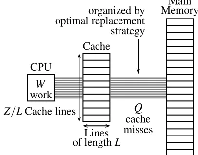
In the ideal-cache model, the processor can only refer to words that reside in the cache. If the referenced line of a word is found in cache, then that word is delivered to the processor for further processing. This situation is literally called a cache hit. Otherwise, a cache miss occurs and the line is first fetched into anywhere in the cache before transferring it to the processor; this mapping from memory to cache is calledfull associativity. If the cache is full, a cache line must be evicted. The ideal cache uses the optimal off-line cache replacement policy to perfectly exploit temporal locality. In this policy, the cache line whose next access is furthest in the future is replaced [2].

(30)

2.12. The ideal cache model 19

f

athena,cel,prokop,sridhar

g

@supertech.lcs.mit.edu

= ( )

( + = )

( +( = )( + )) ( )

( +( + + )= + =

p

)

( ; )

Q

cache misses organized by optimal replacement strategy

Main Memory

Cache

Z=LCache lines

Lines of lengthL

CPU

W

work

>

= ( );

( )

( ; )

Figure 2.1: The ideal-cache model.

This complexity estimate is actually the conventional running time in a RAM model [1]. The second measurement is its cache complexity,Q(n;Z, L), representing the number of cache misses the algorithm incurs as a function of:

• the input data size n, • the cache size Z, and

• the cache line lengthL of the ideal cache.

When Z and L are clear from the context, the cache complexity can be denoted simply byQ(n).

An algorithm whose cache parameters can be tuned, either at compile-time or at run-time, to optimize its cache complexity, is calledcache aware; while other algorithms whose performance does not depend on cache parameters are calledcache oblivious. The performance of a cache-aware algorithm is often satisfactory. However, there are many approaches which can be applied to design optimal cache oblivious algorithms to run on any machine without fine tuning their parameters.

B B

(31)

2.13. Cache complexity of data transposition 20

external-memory bound [14]. However, such type of error is reasonable as our main goal is to match bounds within multiplicative constant factors.

Proposition 1 Scanning n elements stored in a contiguous segment of memory with cache line size L costs at most ⌈n/L⌉ +1 cache misses.

Proof. The main ingredient of the proof is based on the alignment of data elements in memory. We make the following observations.

• Let (q, r) be the quotient and remainder in the integer division of n by L. Let u (resp. wun) be the total number of words in fully (not fully) used cache lines. Thus,

we have n=u+wun.

• If wun = 0 then (q, r) = (⌊n/L⌋,0) and the scanning costs exactly q; thus the

conclusion is clear since⌈n/L⌉ = ⌊n/L⌋in this case.

• If 0<wun <L then (q, r) = (⌊n/L⌋, wun) and the scanning costs exactly q+2; the

conclusion is clear since⌈n/L⌉ = ⌊n/L⌋ +1 in this case.

• If L≤wun<2L then (q, r) = (⌊n/L⌋, wun−L) and the scanning costs exactlyq+1;

the conclusion is clear again.

2.13 Cache complexity of data transposition

We consider the following problem, which plays a fundamental role in implementing multi-dimensional FFTs [24] and TFTs [19]. Given an m×n matrix A stored in a row-major layout, compute and store the transposed matrix AT _{into an}_n×_m _matrix _B _also

stored in a row-major layout. We shall describe a recursive cache-oblivious algorithm which uses Θ(mn) work and incurs Θ(1+mn/L) cache misses, which is optimal. The straightforward algorithm employing doubly nested loops incurs Θ(mn) cache misses on one of the matrices when m≫Z/L and n≫Z/L.

This recursive algorithm due to Leiserson at al. [9] works as follows:

• Ifn≥m, the Rec-Transpose algorithm partitions A= (A1 A2) , B =

⎛ ⎝

B1 B2

⎞ ⎠

and recursively executes Rec−Transpose(A1, B1)and Rec−Transpose(A2, B2). • Ifm>n, the Rec-Transpose algorithm partitions

A=⎛

⎝

A1 A2

⎞

(32)

2.14. Cache complexity of Cooley-Tukey algorithm 21

and recursively executes Rec−Transpose(A1, B1)and Rec−Transpose(A2, B2). The Cilkplus implementation of this algorithm is shown in Section 2.11

2.14 Cache complexity of Cooley-Tukey algorithm

We analyze the cache complexity of the (radix 2) Cooley-Tukey algorithm stated in Section 3.1. for an ideal cache with Z words and L words per cache line. We assume that each coefficient of the input vector fits within a machine word and that the array storing the coefficients consist of consecutive memory words. IfQ(n)denotes the number of cache misses incurred by the algorithm of Section 3.1. then, neglecting misalignment, we have for some 0<α<1,

Q(n) =⎧⎪⎪⎨⎪⎪

⎩

n/L if N <αZ (base case)

2Q(n/2) +n/L if n≥αZ (recurrence) (2.19) Unfolding k times the recurrence relation (2.19) yields

Q(n) =2k_Q₍_n_/₂k_{) +}_kn_/_L.

Assuming n≥αZ and choosing k such that n/2k≃_αZ_{, that is, 2}k ≃ n

αZ, or equivalently

n/L≃2k_αZ/_L_{, we obtain}

Q(n) ≤ 2k_αZ/_L+_kn/_L

= n/L+kn/L

= (k+1)n/L

≤ (log2(αZn ) +1)n/L.

Therefore we haveQ(n) ∈ O(n/L(log2(n)−log2(αZ))). This result is known to be non-optimal, following the work of Hong Jia-Wei and H.T. Kung in their landmark paperI/O complexity: The red-blue pebble game in the proceedings of STOC’81 [14].

Usually, this (non-optimal) radix 2 FFT is implemented as follows:

• If the input vector does not fit in cache, a recursive algorithm is applied

• Once the vector fits in cache, an iterative algorithm (not requiring shuffling) takes over.

(33)

2.15. Blocking strategy for FFT 22

Figure 2.3: Algorithm 3 strategy.

2.15 Blocking strategy for FFT

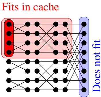
To obtain an optimal FFT in terms of cache-complexity, one should proceed as follows

• Instead of processing row-by-row, one computes as deep as possible while staying in cache (resp. registers): this yields a blocking strategy.

• On the left picture, assumingZ=4, on the first (resp, last) two rows, we successively compute thered,green, blue, orange 4-point blocks.

• On an ideal cache of Z words with L words per cache line the cache complexity drops to O(n/L(log2(n)/log2(Z))) which isoptimal.

This strategy is illustrated by the picture and pseudo-code in Figure 2.4 and is reported in [4]. Figure 2.4 is taken from the Master thesis of Svyatoslav Covanovwww.csd.uwo.ca/

~moreno//Publications/Svyatoslav-Covanov-Rapport-de-Stage-Recherche-2014. pdf. The strategy is used by the BPAS librarywww.bpaslib.org for its FFT code

gen-erator. The work reported in this thesis extends this tool to TFT computations. Our TFT code generator also follows this blocking strategy.

Let us estimate now the cache complexity of the above algorithm for an ideal cache with Z words and L words per cache line. As before, we assume that each coefficient fits within a machine word. If Q(n) denotes the number of cache misses incurred by Algorithm 2, then, neglecting misalignment, we have for some 0<α<1,

Q(n) =⎧⎪⎪⎨⎪⎪

⎩

n/L if n<αZ (base case)

(34)

Figure 2.4: Optimal FFT using blocking.

We shall assume that K <αZ holds. Hence, we have Q(K) ≤K/L. Thus, for n ≥αZ, Relation (2.20) leads to:

Q(n) = KQ(n/K) + 2n/L

≤ Ke_Q(_n/_Ke) + ₂_{e n}/_L

≤ Ke αZ

L + 2e n/L

= n/L(1 + 2e)

≤ n/L3e.

(2.21)

wheree is chosen such that n/Ke=_αZ_{, that is,} _Ke= n

αZ or equivalentlyn/L=K

e_αZ/_L_.

Therefore, we haveQ(n) ∈ O(n/L(logK(n)−logK(αZ))). In particular, forK≃αZ and

since we have

Q(n) ∈ O(n/Llog_αZ(n). (2.22)

(35)

Algorithm 2: FFTradix K(α, ω, n=J⋅K)

Input: α= [a0, a1, . . . , an−1] is the coefficient array of the input polynomial, ω is a

primitive n-th root of unity, n=J⋅K denotesn be split intoK parts of size J.

Output: Array α.

for 0≤j <J do

/* Data transposition */

for 0≤k<K do

γ[j][k] ∶=αkJ+j;

for 0≤j <J do

/* Base case FFTs */

c[j] ∶=FFTbase−case(γ[j], ωJ_{, K})_;

for 0≤k<K do

/* Twiddle factor multiplication */

for 0≤j <J do

δ[k][j] ∶=c[j][k] ∗ωjk _;

for 0≤k<K do

/* Recursive calls */

ζ[k] =FFTradixK(ζ[k], ωK, J);

for 0≤k<K do

/* Data transposition */

for 0≤j<J do

α[jK+k] ∶=ζ[k][j];

return (α0, α1, . . . , αn−1);

Algorithm 3: FFT(α, ω)

Input: α= [a0, a1, . . . , an−1] is the coefficient array of the input polynomial, ω a primitive n-th root of unity.

Output: The output array α becomes

[α0+αn/2, α1+ω⋅αn/2+1, . . . , αn/2−1−ωn/2−1⋅αn−1].

if n≤HT HRESHOLD then

ArrayBitReversal([α0, α1, . . . , αn−1]);

return FFT iterative in cache([α0, α1, . . . , αn−1], ω);

Shuffle([α0, α1, . . . , αn−1]);

[α0, α1, . . . , αn/2−1] =FFT([α0, α1, . . . , αn/2−1], ω2);

[αn/2, αn/2+1, . . . , αn−1] =FFT([αn/2, αn/2+1, . . . , αn−1], ω2);

(36)

Chapter 3 Forward and Inverse Truncated

Fourier Transform

We review the notion of truncated Fourier transform (TFT) as introduced by Joris van der Hoeven in [26], together with detailed pseudo-code and examples for the forward and inverse TFT, follow Paul Vrbik’s tech report about TFT https://carma.newcastle. edu.au/paulvrbik/pdfs/TFT.pdf. We stress the fact those algorithms have the same

specifications as those of David Harvey in [12]. However, the formulation in this latter paper opened the door to conceptually simpler ways of computing TFTs. In fact, David Harvey’s paper inspired the work of Jeremy Johnson and LingChuan Meng [21] which has brought a practically efficient forward TFT algorithm.

In Section 3.1, we review the 2-way divide-and-conquer FFT algorithm presented in Section 2.4. Then, we slightly modify its presentation in order to better introduce the concept of truncated Fourier transform (TFT) in Section 3.2. From there, computing the forward TFT is deduced from the 2-way divide-and-conquer TFT algorithm in a very natural manner: we do this in Section 3.3. Unfortunately, and unlike FFT, the inverse map of TFT is very different from the forward process and, in fact, harder to understand in details. Sections 3.4, 3.5 and 3.6 attempt to deal with this challenge.

3.1 FFT: review and complement

Let R, n, and ω be given as in Section 2.4. The DFT — with respect to ω — of an n-tuple a= (a0, . . . , an−1) ∈Rn is the n-tuple ˆa= (ˆa0, . . . ,aˆn−1) ∈Rn with

ˆ ai=

n−1

∑

j=0

ajωij.

(37)

3.1. FFT: review and complement 26

The n-tuples can alternatively be represented as coefficients of polynomials in_R[x] and the FFT can be defined as the mapping from A = a0 +a1x+ ⋯ +an−1xn−1 to the

n-tuple (A(ω0)_{, . . . , A}(_ωn−1))_{. Binary splitting is used to perform the FFT efficiently by}

evaluating only at ω2i _for _i∈ {₀_{, . . . , e}−₁}_{, rather than all} _ω0_{, . . . , ω}n−1_{. To compute the}

FFT ofa with respect to ω we write

a0, . . . , an−1= (b0, c0, . . . , bn/2−1, cn/2−1)

and compute recursively the Fourier transform of (b0, . . . , bn/2−1) and (c0, . . . , cn/2−1) at

ω2_:

FFTω2(b₀, . . . , b_n/2−1) = (ˆb₀, . . . ,ˆb_n/2−1);

FFTω2(c₀, . . . , c_n/2−1) = (cˆ₀, . . . ,cˆ_n/2−1).

Finally we construct ˆaaccording to

FFTω(a0, . . . , an−1) = (ˆb0+cˆ0, . . . ,ˆbn/2−1+ˆcn/2−1ωn/2−1

ˆ_b₀₋_ˆ_c₀_{, . . . ,}ˆ_b_n_/2−1₋_ˆ_c_n_/2−1_ωn/2−1)_.

The equivalent polynomial interpretation dividesAinto even and odd parts, evaluates them at ω2_{, and then reconstructs to obtain ˆ}_A_{. Although this can be implemented as} a recursive algorithm, it is faster to use avoid the overhead of recursive stacks via an in-place algorithm.

The 2-way divide-and-conquer TFT recalled above can be executed in-place. Let us explain how since this way of presenting Cooley-Tukey algorithm is a good introduction to TFT. We need the following definition.

Definition We denote by [i]e the bit wise reverse1 of i at length e. Suppose i=i020+

⋯ +ie−12e−1 and j =j020+ ⋯ +je−12e−1 then

[i]e=j ⇐⇒ ik=je−k−1 for k∈ {0, . . . , e−1}.

Example [3]5=24 because 3=000112 whose reverse is 110002 =24.

[11]5=26 because 11=010112 whose reverse is 110102=26.

(38)

3.1. FFT: review and complement 27

We begin at step zero with the vector

x0= (x0,0, . . . , x0,n−1) = (a0, . . . , an−1)

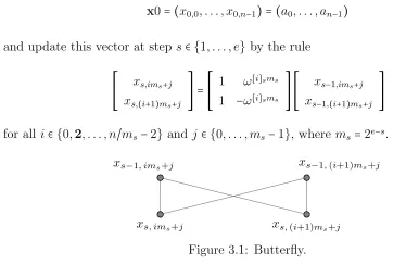
and update this vector at step s∈ {1, . . . , e} by the rule

⎡⎢ ⎢⎢ ⎢⎣

xs,ims+j

xs,(i+1)ms+j

⎤⎥ ⎥⎥ ⎥⎦=

⎡⎢ ⎢⎢ ⎢⎣

1 ω[i]sms

1 −ω[i]sms

⎤⎥ ⎥⎥ ⎥⎦ ⎡⎢ ⎢⎢ ⎢⎣

xs−1,ims+j

xs−1,(i+1)ms+j

⎤⎥ ⎥⎥

⎥⎦ (3.1)

for all i∈ {0,2, . . . , n/ms−2} and j∈ {0, . . . , ms−1}, where ms=2e−s.

xs−1, ims+j xs−1,(i+1)ms+j

xs, ims+j xs,(i+1)ms+j

Figure 3.1: Butterfly.

Figure 3.1, known as a butterfly because of its form, is an illustration of Equation (3.1) as a relation among four values at steps s and s−1. The butterflys width is determined by ms, which decreases as s increases. Note that two additions and one multiplication

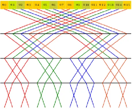
i= 0 i= 1 · · · i= 15

s= 0

s= 1

s= 2

s= 3

s= 4

x3,11

x3,9

x2,11

x2,9

Figure 3.2: Butterflies. Schematic representation of Equation (3.1). The black dots correspond to the xs,i. The top row corresponding tos=0. In this case n=16=24.

are done in Equation (3.1) as one product is merely the negation of the other. Using induction over s, it can be easily shown [26] that

(39)

3.2. The truncated Fourier transform 28

for alli∈ {0, . . . , n/ms−1}and j ∈ {0, . . . , ms−1}. In particular, whens=eand j =0 we

have

xe,i=ˆa[i]e

ˆ

ai =xe,[i]e

for all i∈ {0, . . . , n−1}. That is, ˆa is a permutation ofxe as illustrated in Figure 3.3

a0 a1 a2 a3 a4 a5 a6 a7 a8 a9 a10 a11 a12 a13 a14 a15

b

a[0]4 ba[1]4 ba[2]4 ba[3]4 ba[4]4 ba[5]4 ba[6]4 ba[7]4 ba[8]4 ba[9]4 ba[10]4 ba[11]4 ba[12]4 ba[13]4 ba[14]4 ba[15]4 Figure 3.3: The Fast Fourier Transform for n=16. The top row, corresponding to s=0, represents the values ofx0. The bottom row, corresponding tos=4 is some permutation of ˆa (the result of the FFT on a).

One nice feature of the FFT is that it is straightforward to recover a from ˆa

DFTω−1(aˆ)_i=DFT_ω−1(DFT_ω(a))_i=

n−1

∑

k=0 n−1

∑

j=0

aiω(i−k)j =nai (3.2)

since

n−1

∑

j=0

ω(i−k)j =₀

whenever i ≠ k. This yields a polynomial multiplication algorithm of time complexity O(nlogn)in R[x].

3.2 The truncated Fourier transform

When the length of a (the input) is not equal to a power of two, the `-tuple a =

(a0, . . . , a`−1)is completed by setting ai=0 when i≥` to artificially extend the length of

(40)

3.2. The truncated Fourier transform 29

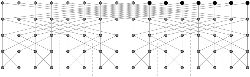
As illustrated in Figures 3.4 and 3.5, FFT will calculate all of ˆa, even if only ` components of ˆa are needed. These unnecessary computations occur when FFT is used to multiply polynomials, as the degree of the product is rarely a power of two.

Figure 3.4: The FFT with “artificial” zero points (green).

Figure 3.5: Removing all unnecessary computations from Figure 3.4 gives the schematic representation of the TFT.

With the exception that the lengths of the input and output vectors (a resp. ˆa) are not necessarily powers of two, the TFT is similar to the FFT. More precisely the TFT of an`-tuple(a0, . . . , a`−1) ∈R` is the `-tuple

(A(ω[0]e ,). . . , A(ω[`−1]e)) ∈R`.

where n=2e_, _`<_n _(usually_`≥_n/_{2) and} _ω _a _n_{-th root of unity.}

Remark A more general description of the TFT, in which one can choose an initial vector (x0,i0, . . . , x0,in) and target vector (xe,j0, . . . , xe,jn), is given by van der Hoeven.

(41)

3.3. Forward TFT: pseudo-code with an illustrative example 30

unnecessary for the desired output if eachikis distinct. However, as we are ignorant to a

sufficiently fast method to find this sub graph, this discussion is restricted to the scenario in which the input and output are the same initial segments, as depicted in Figure 3.5.

The in-place algorithm in the previous section can be easily modified to perform the TFT. At stage s it suffices to compute

(xs,0, . . . , xs,j) with j= (⌊(`−1)/ms⌋ +1)ms−1

where ms=2e−s.2

3.3 Forward TFT: pseudo-code with an illustrative

example

Denote X as a vector overZ/pZ,ω∈Z/pZis a primitive n−th root of unity,pis a prime

number,` is the length ofX,e∶=min{k ∣ `≤2k}_and _n=₂e_{. Initially, we pad the vector}

X (at its end) with zeroes (s. t. its size becomes n) and call it X0. The value of X at the end of the s-th iteration is denoted by Xs for 1≤s≤log2(n). We write xs,i forXs[i]

with 0≤i≤n−1.

Algorithm 4: TFT(X, ω, p)

Input: X is the coefficient array of the input polynomial, ω is a primitiven-th root of unity, pis a prime number

Output: Array X.

for s from 1 to log2n do ms=n/2s

for i from 0 by 2 to (n/ms−2) do

Let is be the bit wise reverse of i in the form of a decimal number

for j from 0 to (ms−1) do

if (i+1)ms+j < ⌈_m`_s⌉ ms then

[ xs,ims+j

xs,(i+1)ms+j

] = [1₁ ₋ω_ωisismmss] [

xs−1,ims+j

xs−1,(i+1)ms+j

]

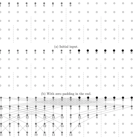
The following is an example of serial forward TFT w.r.t. prime number is 17, ωis 3, ` is 9 andnis 16 which is defined before. The initial input is an vector{1,2,3,4,5,6,7,8,9}.

(42)

3.4. The inverse truncated Fourier transform 31

The size of input ` is 9 and the smallest number which larger than ` and satisfied some power of two is 16. Totally, we need log2n=log216=4 steps to achieve the final output. With zero padding in the end of input to make it a vector {1,2,3,4,5,6,7,8,9,

0,0,0,0,0,0,0}as showing in figure 3.5(b). Using equation 3.1, the second line can be cal-culated from the original input which is an vector {10,2,3,4,5,6,7,8,9,2,3,4,5,6,7,8}.

Applied equation 3.1 to calculate the third line from the second line as before. As showing in the algorithm 2, only ⌈ `

ms⌉ ms items are calculated which is 12 in this step.

After calculation, the output is vector{15,8,10,12,5,13,13,13,6,12,9,6}. Keep applying equation 3.1 to the last two steps and the final output is vector{11,5,4,6,10,15,12,0,13}.

3.4 The inverse truncated Fourier transform

Unlike the FFT, the TFT cannot be inverted simply by performing another TFT with 1/ω and adjusting by a constant factor. There is information missing that must be taken into account.

Example LetR=Z/17Z,n=22 =4, withω=4 an-th primitive root of unity. The TFT

of a= (a0, a1, a2)is

⎡⎢ ⎢⎢ ⎢⎢ ⎢⎣

A(ω0) A(ω2) A(ω1)

⎤⎥ ⎥⎥ ⎥⎥ ⎥⎦= ⎡⎢ ⎢⎢ ⎢⎢ ⎢⎣

A(1) A(−1)

A(3)

⎤⎥ ⎥⎥ ⎥⎥ ⎥⎦= ⎡⎢ ⎢⎢ ⎢⎢ ⎢⎣

a0+a1+a2 a0−a1+a2 a0+3a1+9a2

⎤⎥ ⎥⎥ ⎥⎥ ⎥⎦

Now to show that the TFT of this w.r.t. 1/ω isnot adefine

b= ⎡⎢ ⎢⎢ ⎢⎢ ⎢⎣ b0 b1 b2 ⎤⎥ ⎥⎥ ⎥⎥ ⎥⎦= ⎡⎢ ⎢⎢ ⎢⎢ ⎢⎣

a0+a1+a2 a0−a1+a2 a0+3a1+9a2

⎤⎥ ⎥⎥ ⎥⎥ ⎥⎦

The TFT of b w.r.t 1/ω= −4 is

⎡⎢ ⎢⎢ ⎢⎢ ⎢⎣

B(ω0) B(ω−2) B(ω−1)

⎤⎥ ⎥⎥ ⎥⎥ ⎥⎦= ⎡⎢ ⎢⎢ ⎢⎢ ⎢⎣

B(1) B(−1) B(−4)

⎤⎥ ⎥⎥ ⎥⎥ ⎥⎦= ⎡⎢ ⎢⎢ ⎢⎢ ⎢⎣

b0+b1+b2 b0−b1+b2 b0−4b1−b2

⎤⎥ ⎥⎥ ⎥⎥ ⎥⎦= ⎡⎢ ⎢⎢ ⎢⎢ ⎢⎣

3a0+3a1+11a2 a0+5a1+9a2

−4a0+2a1+5a2

⎤⎥ ⎥⎥ ⎥⎥ ⎥⎦

(43)

3.5. Inverse TFT: an algorithm 32

We follow the paths from xe back tox0 to invert the TFT. If one value of

xs,ims+j, xs−1,ims+j

and one value of

xs,(i+1)ms+j, xs−1,(i+1)ms+j

are known, the other values may be found. In other words, if two values of a butterfly are known, then Equation (3.1) can be used to find the other two values, as the relevant matrix can be inverted. Also, this situation is ideal for implementation, as these relations only involve shifting (multiplication and division by two), additions, subtractions and multiplications by roots of unity.

Given xe,0, . . . , xe,2k₋₁, x_e−_k,₀, . . . , x_e₋_k,₂k₋₁ can be found. As depicted in Figure 3.7,

no butterfly relations necessary to move up in this manner require x_s,₂k+_j for any s ∈

{e−k, . . . , e}, j >0. In general,

x_e,₂j+2k, . . . , x_e,₂j+2k−1

is enough to calculate

xe−k,2j, . . . , x_e−_k,₂j+2k−1

for 0<k≤j<e.

3.5 Inverse TFT: an algorithm

For our restricted case (all padding zeroes packed at the end), a simple recursive descrip-tion of the inverse TFT algorithm is presented. The algorithm operates in a length n array x= (x0, . . . ,xn−1)for which we assume access; here n=2e corresponds to ω, anth

primitive root of unity.

Initially, the content of the array is

x∶= (xe,0, . . . , xe, `−1,0, . . . ,0)

where (xe,0, . . . , xe, `−1) is the result of the TFT on (x0,0, . . . , x0, `−1,0, . . . ,0).

(44)

3.5. Inverse TFT: an algorithm 33

find xs, ims+j. An arrow emphasizes that this new value should also overwrite the one

at xk. With the caveat that i and j are not explicitly known values, this calculation is

easily accomplished using (3.1). As s is known, so arems and an array positionk. Note

i is recovered byi=k quo ms, the quotient of k/ms.

A full description of the inverse TFT follows in Algorithm 5. Note that the initial call is InvTFT(0, `−1, n−1, 1). Figure 3.10 illustrates Algorithm 5.

Algorithm 5: InvTFT(x,head,tail,last, s)

Input: x is an input array, head,tail,last is the indexing of the input array, s=log₂last.

Output: Array x= [x0, x1, . . . , x`].

middle ← last−head

2 +head;

LeftMiddle ← ⌊middle⌋; RightMiddle←LeftMiddle+1;

if head>tail then

Base case—do nothing;

return null;

else if tail≥LeftMiddle then

Push up the self-contained region xhead to xLeftMiddle;

Push down xtail+1 to xlast with ;

InvTFT(x,RightMiddle,tail,last, s+1); s←e−log2(LeftMiddle−head+1);

Push up (in pairs) (xhead,xhead+ms)to (xLeftMiddle,xLeftMiddle+ms) with ; else if tail<LeftMiddle then

Push down xtail+1 to xLeftMiddle with ;

(45)

3.6. Illustration of the inverse TFT algorithm 34

3.6 Illustration of the inverse TFT algorithm

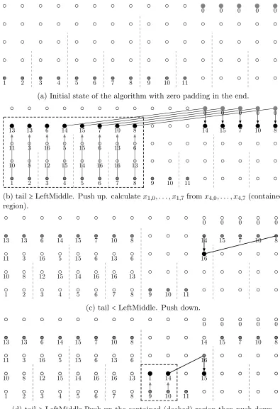
Figure 3.11 and Figure 3.12 show an example of the inverse TFT algorithm w.r.t prime number is 17,ωis 3,`is 11 andnis 16. The initial input is an vector{1,2,3,4,5,6,7,8,9, 10,11}in the first step and zero padding in the final step. The algorithm operates on a length-n array X = (X[0], . . . , X[n−1]) with n=2e_{, 1}≤_`<_n _{(the last} _n−_` _coefficients

being zeroes) and ω is an n-th primitive root of unity). Thus, initially, the contents of the array are

X= (xe,0, . . . , xe,`−1,0, . . . ,0)

where (xe,0, . . . , xe,`−1) is the result of the TFT on (x0,0, . . . , x0,`−1,0, . . . ,0), ultimately,

the output of the computation.

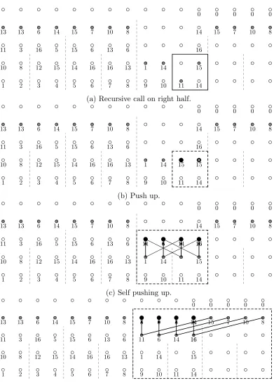
According to Algorithm 4, tail≥LeftMiddle (tail=10, LeftMiddle=7) self-contained push up is used to calculate x1,0, . . . , x1,7 from x4,0, . . . , x4,7 using Equation 3.1. Then push down xtail+1 to xlast which is x4,11 to x4,15 here. After calculation,x4,11 to x4,15 is equal to {14,15,7,10,8}.

Recursive call on right half. Tail ≤ LeftMiddle (tail =2, LeftMiddle=3), push down to calculate x3,11=16. Recursive call on left half. Tail≥LeftMiddle (tail=2, LeftMiddle

=1), push up the contained (dashed) region then push down. After calculation,x2,8 =1, x2,9=14 and x2,11=15. Recursive call on right half to obtain x2,10=15.

Following Algorithm 5, do pushing up to calculatex3,8 tox3,11 which is{11,6,14,16}. Self push up to calculate x4,8 to x4,11 which is {3,0,3,14}.

(46)

1 2 3 4 5 6 7 8 9

(a) Initial input.

1 2 3 4 5 6 7 8 9 0 0 0 0 0 0 0

(b) With zero padding in the end.

1 2 3 4 5 6 7 8 9 0 0 0 0 0 0 0

10 2 3 4 5 6 7 8 9 2 3 4 5 6 7 8

15 8 10 12 5 13 13 13 6 12 9 6

8 3 5 13 4 12 6 14 2 15

11 5 4 6 10 15 12 0 13

(c) Values of each step.

Figure 3.6: Example of TFT where n=16, `=9, prime number is 17, and ω=3.

xk=xs−1, ims+j xs−1,(i+1)ms+j =xk+ms+j

xs, ims+j xs,(i+1)ms+j

(47)

xhead xtail

xlast

2n ₂n

s=p−n−1

s=p−n

s=p

(a) Line (8): push up the self contained (dashed) region. This yields values sufficient to push down at line (9).

xhead xtail

xlast

2n

s=p−n−1

s=p−n

s=p

(b) This enables us to make a recursive call on the dashed region (line (12)). By our induction hypothesis this brings all points at s=p tos=p−n.

s=p−n−1

s=p−n

s=p

(c) Sufficient points ats=p−n are known to move tos=p−n−1 at line (13).

(48)

xhead xtail

xlast

2n ₂n

s=p−n−1

s=p−n

s=p

(a) Initially there is sufficient information to push down at line (14).

xhead xtail

xlast

2n ₂n

s=p−n−1

s=p−n

s=p

(b) This enables us to make the prescribed recursive call at line (15).

2n ₂n

s=p−n−1

s=p−n

s=p

(c) By the induction hypothesis this brings the values in the dashed region tos=p−n, leaving

enough information to move up at line (16).

(49)

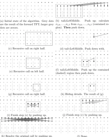
(a) Initial state of the algorithm. Grey dots are the result of the forward TFT; larger grey dots are zeroes.

(b) tail≥LeftMiddle. Push up; calculate

x1,0, . . . , x1,7 fromx4,0, . . . , x4,7 (contained re-gion). Thenpush down.

(c) Recursive call on right half. (d) tail<LeftMiddle. Push down with.

(e) Recursive call on left half. (f) tail≥LeftMiddle. Push up the contained (dashed) region then push down.

(g) Recursive call on right half. (h) Hiding details. The result of (g).

(i) Finish step (e) by pushing up. (j) Finish step (c) by pushing up.

(k) Resolve the original call by pushing up. (l) Done.

(50)

0 0 0 0 0

1 2 3 4 5 6 7 8 9 10 11

(a) Initial state of the algorithm with zero padding in the end.

0 0 0 0 0

1 2 3 4 5 6 7 8 9 10 11 10 8 12 15 14 16 16 13

11 3 16 5 15 6 13 6

13 13 6 14 15 7 10 8 14 15 7 10 8

(b) tail≥LeftMiddle. Push up. calculatex₁_,₀, . . . , x₁_,₇ fromx₄_,₀, . . . , x₄_,₇ (contained

region).

0 0 0 0 0

1 2 3 4 5 6 7 8 9 10 11 10 8 12 15 14 16 16 13

11 3 16 5 15 6 13 6

13 13 6 14 15 7 10 8 14 15 7 10 8

16

(c) tail <LeftMiddle. Push down.

0 0 0 0 0

1 2 3 4 5 6 7 8 9 10 11 10 8 12 15 14 16 16 13

11 3 16 5 15 6 13 6

13 13 6 14 15 7 10 8 14 15 7 10 8

16

1 14 15

(d) tail ≥LeftMiddle.Push up the contained (dashed) region then push down.

Implementation Techniques for the Truncated Fourier Transform

Scholarship@Western

Scholarship@Western

Implementation Techniques for the Truncated Fourier Transform

Implementation Techniques for the Truncated Fourier Transform

IMPLEMENTATION TECHNIQUES FOR THE TRUNCATED

FOURIER TRANSFORM

Li Zhang

Graduate Program in Computer Science

October 26, 2015

The School of Graduate and Postdoctoral Studies

The University of Western Ontario

London, Ontario, Canada

Abstract

Acknowledgments

Contents

List of Algorithms

List of Tables

List of Figures

Chapter 1

Introduction

1.1

Literature review

1.2

Contributions of this thesis

Chapter 2

Background

2.1

Rings and fields

2.2

Montgomery arithmetic

2.3

Primitive roots of unity

2.4

Discrete Fourier transform (DFT)

2.5

Fast Fourier transform (FFT)

2.6

Montgomery arithmetic in practice

2.7

Tensor algebra

2.8

Cooley Tukey factorization formula

2.9

Multi-core architectures

2.10

The fork-join concurrency model

2.11

The CilkPlus programming language

2.12

The ideal cache model

athena,cel,prokop,sridhar

@supertech.lcs.mit.edu

2.13

Cache complexity of data transposition

2.14

Cache complexity of Cooley-Tukey algorithm

2.15

Blocking strategy for FFT

Chapter 3

Forward and Inverse Truncated

Fourier Transform

3.1

FFT: review and complement

3.2

The truncated Fourier transform

3.3

Forward TFT: pseudo-code with an illustrative

example

3.4

The inverse truncated Fourier transform

3.5

Inverse TFT: an algorithm

3.6

Illustration of the inverse TFT algorithm