Statistical methods for the analysis of RNA sequencing data

(1)

Scholarship@Western

Electronic Thesis and Dissertation Repository

3-27-2014 12:00 AM

Statistical methods for the analysis of RNA sequencing data

Man-Kee Maggie Chu

The University of Western Ontario

Supervisor Dr. Wenqing He

The University of Western Ontario

Graduate Program in Statistics and Actuarial Sciences

A thesis submitted in partial fulfillment of the requirements for the degree in Doctor of Philosophy

Follow this and additional works at: https://ir.lib.uwo.ca/etd

Part of the Biostatistics Commons, and the Longitudinal Data Analysis and Time Series Commons

Recommended Citation Recommended Citation

Chu, Man-Kee Maggie, "Statistical methods for the analysis of RNA sequencing data" (2014). Electronic Thesis and Dissertation Repository. 1935.

https://ir.lib.uwo.ca/etd/1935

This Dissertation/Thesis is brought to you for free and open access by Scholarship@Western. It has been accepted for inclusion in Electronic Thesis and Dissertation Repository by an authorized administrator of

(2)

(Thesis format: Monograph)

by

Man-Kee Maggie Chu

Graduate Program in Statistical and Actuarial Sciences

A thesis submitted in partial fulfillment

of the requirements for the degree of

Doctor of Philosophy

The School of Graduate and Postdoctoral Studies

The University of Western Ontario

London, Ontario, Canada

c

(3)

The next generation sequencing technology, RNA-sequencing (RNA-seq), has an increas-ing popularity over traditional microarrays in transcriptome analyses. Statistical methods used for gene expression analyses with these two technologies are different because the array-based technology measures intensities using continuous distributions, whereas RNA-seq provides absolute quantification of gene expression using counts of reads. There is a need for reliable statistical methods to exploit the information from the rapidly evolving sequencing technolo-gies and limited work has been done on expression analysis of time-course RNA-seq data.

Functional clustering is an important method for examining gene expression patterns and thus discovering co-expressed genes to better understand the biological systems. Clustering-based approaches to analyze repeated digital gene expression measures are in demand. In this dissertation, we propose a model-based clustering method for identifying gene expression pat-terns in time-course RNA-seq data. Our approach employs a longitudinal negative binomial mixture model to postulate the over-dispersed time-course gene count data. The effectiveness of the proposed clustering method is assessed using simulated data and is illustrated by real data from time-course genomic experiments.

Due to the complexity and size of genomic data, the choice of good starting values is an important issue to the proposed clustering algorithm. There is a need for a reliable initialization strategy for cluster-wise regression specifically for time-course discrete count data. We modify existing common initialization procedures to suit our model-based clustering algorithm and the procedures are evaluated through a simulation study on artificial datasets and are applied to real genomic examples to identify the optimal initialization method.

Another common issue in gene expression analysis is the presence of missing values in the datasets. Various treatments to missing values in genomic datasets have been developed but limited work has been done on RNA-seq data. In the current work, we examine the per-formance of various imputation methods and their impact on the clustering of time-course RNA-seq data. We develop a cluster-based imputation method which is specifically suitable for dealing with missing values in RNA-seq datasets. Simulation studies are provided to assess the performance of the proposed imputation approach.

Keywords: RNA-seq data, time-course, cluster analysis, missing values

(4)

(5)

I would like to thank my supervisor Dr. Wenqing He for his continuous guidance during my studies. This research would not have been possible without his support and encouragement. I am also very grateful of everyone in the Department of Statistical and Actuarial Sciences at the University of Western Ontario for their academic and logistic support throughout the years. I want to extend my appreciation to the faculty members for their academic advices and the friendly staff Jane, Jennifer and Lisa for their assistance. I would also like to thank my col-leagues in the department for their friendship and support.

I want to thank my parents for their unconditional love for me. Without their encour-agement and support, I would never have been able to pursue my interests and achieve this accomplishment. Also, my heartfelt love and thanks go to my fiance Thaddeus for his love and support during my time in graduate school.

(6)

Abstract ii

Dedication iii

Acknowlegements iv

List of Figures viii

List of Tables x

1 Introduction and Background 1

1.1 Motivation . . . 1

1.2 Background knowledge . . . 2

1.2.1 Gene expression analysis . . . 2

1.2.2 Microarrays . . . 2

1.2.3 Gene expression by sequencing . . . 4

1.2.4 RNA-seq . . . 6

1.2.5 Microarrays vs. RNA-seq . . . 10

1.3 Example datasets . . . 13

1.3.1 Fibroblast data . . . 13

1.3.2 Fruit flies data . . . 14

1.4 Existing methodology for gene expression analysis of RNA-seq data . . . 15

1.5 Existing methodology for treatments of missing values . . . 21

1.5.1 Imputation methods for missing values in gene expression data . . . 21

Impact of imputation on gene analysis . . . 24

1.6 Objectives and statement of problems . . . 25

1.6.1 Functional clustering for time-course genomic data . . . 25

1.6.2 Initialization procedures for finite mixture models . . . 26

1.6.3 Missing value imputation methods for clustering of time-course ge-nomic data . . . 28

1.7 Organization of dissertation . . . 29

2 Clustering of time-course RNA-seq data 30 2.1 Introduction . . . 30

2.1.1 Cluster analysis . . . 31

(7)

2.1.3 Clustering of time-course RNA-seq data . . . 38

2.2 Model . . . 41

2.2.1 Mixture models . . . 41

2.2.2 Mixture models: Discrete longitudinal count data . . . 43

2.2.3 Estimation . . . 46

2.2.4 The Property of the Proposed Method . . . 50

2.3 Simulation study . . . 53

2.3.1 Data generation . . . 54

2.3.2 Estimation algorithms . . . 54

2.3.3 Results . . . 56

Two-component mixtures . . . 56

Four-component mixtures . . . 63

Model selection . . . 67

Model misspecification . . . 69

2.4 Real data analysis . . . 71

2.5 Summary . . . 87

3 Initialization procedures for EM estimation of finite mixture models 88 3.1 Introduction . . . 88

3.1.1 Starting values for cluster analysis . . . 89

3.2 Method: Initialization strategies . . . 92

3.3 Simulation study . . . 93

3.3.1 Results . . . 96

Varying dispersion parameter . . . 96

Varying percent of sampling . . . 105

3.4 Real data analysis . . . 111

3.5 Summary . . . 113

4 Missing Data in high-dimensional datasets 115 4.1 Introduction . . . 115

4.1.1 Missing mechanism and treatments of missing values . . . 116

4.2 Methods . . . 118

4.2.1 Imputation methods . . . 118

4.2.2 Datasets and missing data . . . 119

4.2.3 Results . . . 121

MCAR simulated data . . . 121

MAR simulated data . . . 124

MCAR fruit flies data . . . 126

(8)

4.3.1 Results from clustering . . . 138

Datasets with MCAR missingness . . . 138

Datasets with MAR missingness . . . 140

4.3.2 Discussion . . . 142

4.4 Cluster-based imputation method . . . 146

4.4.1 Model . . . 146

4.4.2 Data and evaluation . . . 148

4.4.3 Results . . . 148

4.4.4 Discussion . . . 151

5 Conclusions and future work 154

Bibliography 158

Curriculum Vitae 170

(9)

1.1 The central dogma: Transcription of DNA to RNA to protein . . . 3

1.2 Control of gene expression . . . 4

1.3 Microarray experiment workflow . . . 5

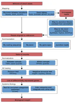
1.4 Overview of RNA-seq experiment and data analysis process (Wang et al., 2010) 7 1.5 Overview of RNA-seq analysis pipeline for detecting differential expression (Oshlack et al., 2010) . . . 8

2.1 Simulation cases: Combinations of trajectories. . . 55

2.2 True and estimated trajectories for Case 4 (s= 2). . . 62

2.3 Simulated trajectories for the four-component mixtures. . . 65

2.4 Four-component mixtures: Estimated trajectories by EM (dispersion=10). . . . 66

2.5 Four-component mixtures: Adjusted Rand Index (ARI) (with varying disper-sion parameters). . . 67

2.6 Four-component mixtures: Percent of correctly classified genes (with varying dispersion parameters). . . 68

2.7 Four-component mixtures: Adjusted Rand Index (ARI) when model is mis-specified and data generated from negative binomial distributions with varying dispersion parameter . . . 71

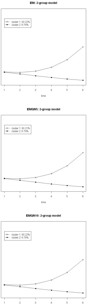
2.8 Fibroblast data: two-component models. . . 74

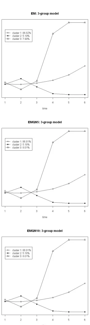
2.9 Fibroblast data: three-component models. . . 75

2.10 Fibroblast data: four-component models. . . 76

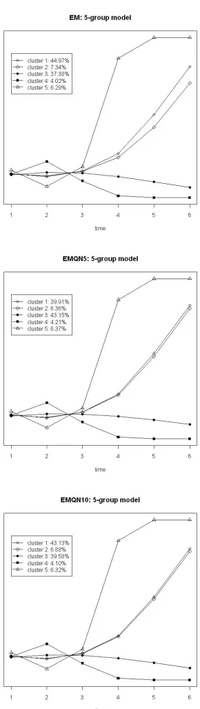
2.11 Fibroblast data: five-component models. . . 77

2.12 Fibroblast data: six-component models. . . 78

2.13 Fruit flies data: two-component models. . . 82

2.14 Fruit flies data: three-component models. . . 83

2.15 Fruit flies data: four-component models. . . 84

2.16 Fruit flies data: five-component models. . . 85

2.17 Fruit flies data: six-component models. . . 86

3.1 Mean ARI of the different initialization strategies across the three dispersion parameter settings. . . 98

3.2 Mean ARI of the different initialization strategies across the three dispersion parameter settings (excluding datasets with non-identifiable models). . . 99

4.1 Schematic illustration of the simulation study: evaluation by RMSE comparing accuracy of imputation methods. . . 121

(10)

4.3 MCAR simulated data: RMSE obtained by KNNimpute whenkranges from 5 to 100. . . 123 4.4 MCAR simulated data: RMSE obtained by SVDimpute with variousk

param-eter across different missing probabilities. . . 124 4.5 MCAR simulated data: RMSE obtained by SVDimpute whenkranges from 1

to 5. . . 125 4.6 MAR simulated data: RMSE obtained by KNNimpute with variouskparameter

across different missing probabilities. . . 126 4.7 MAR simulated data: RMSE obtained by KNNimpute whenk ranges from 5

to 100. . . 127 4.8 MAR simulated data: RMSE obtained by SVDimpute with variouskparameter

across different missing probabilities. . . 128 4.9 MAR simulated data: RMSE obtained by SVDimpute whenkranges from 1 to 5.129 4.10 MCAR fruit flies data: RMSE obtained by KNNimpute with variousk

param-eter across different missing probabilities. . . 130 4.11 MCAR fruit flies data: RMSE obtained by KNNimpute whenkranges from 5

to 100. . . 131 4.12 MCAR fruit flies data: RMSE obtained by SVDimpute with variousk

parame-ter across different missing probabilities. . . 132 4.13 MCAR fruit flies data: RMSE obtained by SVDimpute whenk ranges from 1

to 6. . . 133 4.14 MAR fruit flies data: RMSE obtained by KNNimpute with variouskparameter

across different missing probabilities. . . 134 4.15 MAR fruit flies data: RMSE obtained by KNNimpute whenkranges from 5 to

100. . . 135 4.16 MAR fruit flies data: RMSE obtained by SVDimpute with variouskparameter

across different missing probabilities. . . 135 4.17 MAR fruit flies data: RMSE obtained by SVDimpute whenkranges from 1 to 5. 136 4.18 MCAR simulated data: mean ARI resulted from clustering datasets with 1%,

5% and 10% missing entries (excluding datasets with non-identifiable models). 144 4.19 MAR simulated data: mean ARI resulted from clustering datasets with 1%, 5%

and 10% missing entries (excluding datasets with non-identifiable models). . . 145

(11)

2.1 Lower and upper bounds specified for quasi-Newton estimation. . . 56

2.2 Number of datasets included in analysis. . . 57

2.3 Relative bias of mean estimated mixing proportions. . . 58

2.4 Relative bias of mean parameter estimates for Case 1. . . 58

2.8 Contingency table for comparing two partitionsU andV. . . 64

2.9 BIC values: EM estimation for four-component mixtures . . . 68

2.10 Fibroblast data: BIC values for models. . . 72

2.11 Fruit flies data: BIC values for models. . . 79

3.1 Run-time required for the different initialization strategies. . . 97

3.2 Number of datasets included, mean Adjusted Rand Index (standard deviation), mean percent correctness (standard deviation), and mean EM iterations re-quired for the different initialization strategies (including all 500 datasets) when s=10. . . 100

3.3 Number of datasets included, mean Adjusted Rand Index (standard deviation), mean percent correctness (standard deviation), and mean EM iterations re-quired for the different initialization strategies (excluding datasets with non-identifiable models) whens= 10. . . 101

3.5 Number of datasets included, mean Adjusted Rand Index (standard deviation), mean percent correctness (standard deviation), and mean EM iterations re-quired for the different initialization strategies (excluding datasets with non-identifiable models) whens= 5. . . 105

(12)

quired for the different initialization strategies (excluding datasets with non-identifiable models) whens= 2. . . 107 3.8 Run-time required for the various initialization procedures with sampling

com-ponents (10%, 30% and 50% of sampling). . . 108 3.9 Number of datasets included, mean Adjusted Rand Index (standard deviation),

mean percent correctness (standard deviation) and mean EM iterations required for the different sampling initialization strategies across various sampling per-centages. . . 109 3.10 Number of datasets included, mean Adjusted Rand Index (standard deviation),

mean percent correctness (standard deviation) and mean EM iterations required for the different sampling initialization strategies across various sampling per-centages (excluding datasets with non-identifiable models). . . 110 3.11 Results of initialization strategies used on the fibroblasts data using mixtures

of negative binomials with four components. . . 112 3.12 Results of initialization strategies used on the fruit flies data using mixtures of

negative binomials with four components. . . 113 4.1 MCAR simulated data: Comparison of RMSE of the imputation methods (means

and standard deviations of 500 simulation runs). . . 123 4.2 MAR simulated data: Comparison of RMSE of the imputation methods (means

and standard deviations of 500 simulation runs). . . 127 4.3 MCAR fruit flies data: Comparison of RMSE of the imputation methods (means

and standard deviations of 500 simulation runs). . . 131 4.4 MAR fruit flies data: Comparison of RMSE of the imputation methods (means

and standard deviations of 500 simulation runs). . . 132 4.5 Number of datasets included, mean ARI (standard deviation), mean percent

correctness (standard deviation), and mean EM iterations required for the clus-tering with various imputation methods for datasets with MCAR at 1%. . . 140 4.6 Number of datasets included, mean ARI (standard deviation), mean percent

correctness (standard deviation), and mean EM iterations required for the clus-tering with various imputation methods for datasets with MAR at 1%. . . 142 4.9 Number of datasets included, mean ARI (standard deviation), mean percent

correctness (standard deviation), and mean EM iterations required for the clus-tering with various imputation methods for datasets with MAR at 5%. . . 142 4.10 Number of datasets included, mean ARI (standard deviation), mean percent

correctness (standard deviation), and mean EM iterations required for the clus-tering with various imputation methods for datasets with MAR at 10%. . . 143

(13)

probabilities. . . 149 4.12 MAR simulated data: mean RMSE (and standard deviations) obtained by

cluster-based imputation and other imputation methods across different missing prob-abilities. . . 150 4.13 MCAR fruit flies data: mean RMSE (and standard deviations) obtained by

cluster-based imputation and other imputation methods across different missing probabilities. . . 151 4.14 MAR fruit flies data: mean RMSE (and standard deviations) obtained by

cluster-based imputation and other imputation methods across different missing prob-abilities. . . 152

(14)

Introduction and Background

1.1 Motivation

In order to have a better understanding of complex conditions such as heart disease and can-cers, there is a need for advancements in identifying genes related to common chronic diseases. This can be achieved by furthering our knowledge of gene functions through statistical models, such as performing statistical analysis of gene expression profiles. Since the mid-1990s, DNA microarrays have been the technology of choice for studying gene expression levels. However, these methods have several limitations which restrict their uses in genome research.

Recently, next-generation sequencing technologies have increased sequencing capacity at a fast rate such that ultra-high-throughput sequencing is emerging as the preferred approach over hybridization-based microarrays for characterizing and quantifying entire genomes. As the cost of sequencing continues to fall, the more powerful sequencing data is expected to re-place microarrays for many applications. However, there is a need for reliable and accurate statistical analysis methods to exploit the information carried by the rapidly evolving sequenc-ing technologies.

(15)

1.2 Background knowledge

1.2.1 Gene expression analysis

The production of proteins in a biological system is controlled by genes through transcription and translation. This production process is referred to the central dogma of molecular biology and it is illustrated in Figure 1.1. Transcription refers to the process of messenger ribonucleic acid (mRNA) being copied and edited from the deoxyribonucleic acid (DNA) coding of the gene and translation represents the assembly of amino acids from mRNA to form the protein (Parmigiani et al, 2003). Cellular activity is controlled by the amount of mRNA being tran-scribed or expressed by individual genes, and gene expression can be controlled at different steps (see Figure 1.2). Gene regulation is necessary because cells can prevent resources be-ing wasted by switchbe-ing offgenes that are not needed, and gene activity is controlled first and foremost at the transcription stage. Since the main site of control for most cells is the reg-ulation of transcription, exploring the RNA component of cells, known as the transcriptome, can provide great insight into the biological system as a whole. Some of the techniques avail-able for measuring gene expression levels include serial analysis of gene expression (SAGE), complementary DNA (cDNA) subtraction, differential display, cDNA-sequencing, multiplex quantitative reverse transcription polymerase chain reaction (RT-PCR), and microarrays. The most popular methods used in gene expression investigations are microarrays and cDNA li-brary sequencing.

1.2.2 Microarrays

(16)

Figure 1.1:The central dogma: Transcription of DNA to RNA to protein

This dogma forms the backbone of molecular biology and is represented by four major stages. (1) The DNA replicates its information in a process that involves many enzymes: replication. (2) The DNA codes for the production of messenger RNA (mRNA) during transcription. (3) In eucaryotic cells, the mRNA is processed (essentially by splicing) and migrates from the nucleus to the cytoplasm. (4) Messenger RNA carries coded information to ribosomes. The ribosomes “read” this information and use it for protein synthesis. This process is called translation. Proteins do not code for the production of protein, RNA or DNA. They are involved in almost all biological activities, structural or enzymatic. (Public domain image from Access Excellence @ the National Health Museum, http://www.accessexcellence.org/RC/VL/GG/images/central.gif)

(17)

Figure 1.2:Control of gene expression

Eukaryotic gene expression can be controlled at several different steps. Examples of regulation at each of the steps are known, although for most genes the main site of control is step 1- transcription of a DNA sequence into RNA. (Public domain image from Access Excellence @ the National Health Museum, http://www.accessexcellence.org/RC/VL/GG/ecb/ecb images/08 03 gene expression.jpg)

1.2.3 Gene expression by sequencing

Another widely used method for exploring transcriptomes is by the advanced DNA-sequencing technology. Microarray has been the technology of choice for gene expression investigations since the mid-1990s, but the Sanger sequencing biochemistry (Sanger et al., 1977) quickly set the stage for sequencing to become an attractive alternative technology for biological research.

(18)

se-Figure 1.3:Microarray experiment workflow

(Public domain image from Genomic Research Laboratory, Geneva, http://www.genomic.ch/pict/workflow.png)

quences from both the publicly funded project and Celera were published in 2001 (Lander et al., 2001; Venter et al., 2001).

With the success of HGP, very large-scale sequencing of genome is now the approach for analyzing many problems concerning biology, disease and the environment. As an advance-ment from the ’first generation’ Sanger method, next generation sequencing (NGS) methods were developed to produce an enormous amount of data rapidly and cheaply. These NGS meth-ods, including systems from 454 Life Sciences (Roche) (Margulies et al., 2005), Illumina GA (formerly Solexa) (Bennett et al. 2005), and Applied Biosystems’ SOLiD

(19)

extraction from each feature as compared to the Sanger method, but the parallelized nature of the process provides much higher total throughput with lower cost by generating thousands of bases per second. Also, by over sampling the single fragments during sequencing, these novel methods may offer greater coverage and increased total accuracy when attempting to build the original sequence (Pettersson et al., 2009).

The development of ultra-high-throughput sequencing technologies with decreased cost in recent years allow for numerous applications in biological research (Shendure and Ji, 2008). Gene expression analysis with whole-transcriptome sequencing (RNA-Seq) can be performed to determine quantitative differences between samples and for annotation of splice junctions and transcript boundaries. Other applications of sequencing technologies include detecting the presence of an event such as the binding of a transcription factor, full-genome resequencing for discovery of mutations or polymorphisms, mapping of copy number variation, analysis of DNA methylation and genome-wide mapping of DNA-protein interactions (ChIP-Seq analy-ses).

1.2.4 RNA-seq

In RNA-seq experiments, a sample of purified RNA is first sheared and converted into cDNA, then sequenced on a high-throughput platform such as Illumina, SOLiD or Roche454. The platforms differ in their biochemistry and processing steps, but they all generate millions of short reads either taken from one end or from both ends of each cDNA fragment as results. An overview of a general RNA-seq experiment is described in Figure 1.4a, and the data analysis process illustrated in Figure 1.4b is general for gene expression analysis or discovery of novel gene and alternative splicing.

(20)

and the steps for detecting differences in gene expression levels between samples in RNA-seq would then follow the processing pipeline outlined in Oshlack et al. (2010) and illustrated in Figure 1.5. To measure gene expression (or transcript abundance), the sequencing reads ob-tained are aligned to a known reference genome sequence, and the proportion of reads match-ing a given transcript is used as quantification of its expression level and followed by statistical testing of difference in quantification values between samples (Oshlack et al, 2010, Bloom et al, 2009).

Figure 1.4: Overview of RNA-seq experiment and data analysis process (Wang et al., 2010)

(21)

Figure 1.5:Overview of RNA-seq analysis pipeline for detecting differential expression (Oshlack et al., 2010)

as single-nucleotide polymorphisms (SNPs, variations occurring in individual nucleotides) and insertions or deletions (indels). Also, the short reads can sometimes be aligned to multiple locations on the reference and the presence of sequencing errors also needs to be accounted for (Oshlack et al., 2010).

(22)

outside the annotated exons (Oshlack et al., 2010). There are other alternative approaches of summarization such as including reads along the whole gene length to incorporate reads from introns or including only reads that map to coding sequences (Trapnell et al., 2009). With these various options of summarization methods, the count for each gene may change substantially but little research has been done to determine the optimal method for DE analysis.

The follow step involves normalizing the summarized data, which has been shown to be crucial in DE analysis with RNA-seq data (Anders and Huber, 2010; Bullard et al., 2010; Robinson and Oshlack, 2010). Different normalization methods can be used in order for accu-rate within- and between-sample comparisons of expression levels. To quantify the expression levels of genes within the sample, a widely used approach is to use RPKM (reads per kilobase of exon model per million mapped reads). It is known that longer transcripts are associated with higher read counts at the same expression level, so normalization using RPKM would take into account this gene length effect by dividing the summarized counts by the length of the gene (Marioni et al., 2008; Mortazavi et al., 2008).

(23)

Oshlack, 2010), performing quantile normalization or employing a method which usess match-ing power law distributions (Balwierz et al., 2009). However, the latter two methods may not be appropriate for testing DE since these non-linear transformations remove the count nature of the data and that quantile normalization cannot improve DE detection to the same extent as an appropriate scaling factor (Bullard et al., 2010).

The last step of a DE analysis often involves performing statistical testing between sam-ples of interest using the table of summarized count data for each library after normalization. In general, the Poisson distribution may be used to model the RNA-seq count data, but the Poisson assumption does not account for biological variability in the data (Nagalakshmi et al., 2008; Robinson and Smyth, 2007). Ignoring this issue on datasets with biological replicates will result in false positive rates due to underestimation of sampling error (Anders and Huber, 2010). The negative binomial distribution, which requires an additional dispersion parameter to be estimated, is often used to deal with the biological variability in the data. Variations of negative-binomial-based DE analysis of count data have been proposed (Anders and Huber, 2010; Hardcastle and Kelly, 2010; Robinson and Smyth, 2008), along with models which ex-tend the Poisson model by including over-dispersion (Srivastava and Chen, 2010). It is worth noting that these current strategies target data from simple experimental designs. For analysis of more complex designs such as paired samples or time-course experiments, further research is required to develop such methods in the context of RNA-seq data.

1.2.5 Microarrays vs. RNA-seq

(24)

gives discrete measurement of reads for each gene. Although the underlying methods for mea-suring expression are different, studies have demonstrated that the estimated expression levels have good agreement between the two technologies with correlations ranging from 0.62-0.75 and little variation within methods (Fu et al., 2009; Marioni et al., 2008; Mortazavi et al., 2008).

Transcriptome studies are switching to rely on sequencing-based methods rather than mi-croarrays since RNA-seq has higher sensitivity and dynamic range, with lower technical vari-ation and thus higher precision than microarrays (Bradford et al., 2010; ’t Hoen et al., 2008; Oshlack et al., 2010). In comparison to analysis of array data at the same false discovery rate, more differentially expressed genes could be identified by using sequenced data (Marioni et al., 2008). Sequencing-based methods have another advantage of quantifying expression levels in digital, rather than analog, measurements, as the absolute read counts they provide would allow for highly reproducible comparison of transcripts among and within samples or technical replicates (Matukumalli and Schroeder, 2009; Mortazavi et al., 2008).

(25)

hybridization techniques rely on specific signal-to-noise ratio threshold of the array fluores-cence to be established in order to detect rare transcripts, and background hybridization levels especially limit the precision of expression measurements for transcripts which are in low abun-dance (Marioni et al., 2008; Matukumalli and Schroeder, 2009; Mortazavi et al., 2008).

In regards to the detection of previously unmapped genes and RNA splice events, dense whole-genome tiling microarrays can be used but it is not an attractive method due to the requirement of large amounts of input RNA and other limitations that affect direct splice de-tection (Mortazavi et al., 2008). On the other hand, sequencing technology is superior over microarrays due to its ability to provide details on novel transcribed regions, alternative splic-ing and editsplic-ing of RNA, and allele-specific expression. Microarray probes are only designed to cover small portion of a gene so it is not possible to detect novel transcribed regions, whereas RNA-seq does not rely on pre-determined probes and can be performed on any species lack-ing both the genome sequence and gene content, allowlack-ing it to be used for detectlack-ing novel transcription at previously uncharacterized loci (Bradford et al. 2010; Marioni et al., 2008; Matukumalli and Schroeder, 2009; Mortazavi et al., 2008). Sequencing-based methods can not only explore novel gene content, they can also characterize splicing events by capturing reads that span exon-exon junctions, and examine splice variants and rare transcripts (Bradford et al., 2010; Fu et al., 2009; Marioni et al., 2008; Matukumalli and Schroeder, 2009).

(26)

its mutated form matching to another existing sequence in the genome, leading to false-positive results in seq (Mortazavi et al., 2008; Oshlack et al., 2010). Other weaknesses of RNA-seq include ambiguous mapping for paralogous RNA-sequences and GC content bias (Bloom et al., 2009; Bullard et al., 2010; Mortazavi et al., 2008). Paralogous genes (diverged genes after a duplication event) often occur in large genomes and the process of mapping reads need to take into account of the multiple matching sites in the genome. The sensitivity and accuracy of sequencing-based methods rely on having significant read coverage over the genome with enough detail for low abundance transcript, but less information is available for genes at a low expression level thus the methods are often biased (Bloom et al., 2009; Bradford et al., 2010; Mortazavi et al., 2008).

Technical constraints, cost, throughput and ease of data analyses are all aspects of genome analyses which need to be well-balanced. For different transcript-profiling platforms, their sen-sitivity, accuracy and coverage all need to be taken into consideration when trying to select the optimal technology for the problem of interest. A major concern of RNA-seq has been the costs of the experiments. However, the expenses of sequencing methods will continue to de-crease as technology improves, with increasing number of reads being generated from a single sequencing run and allowing for multiple samples to be processed simultaneously. RNA-seq will continue to gain strength as a transcriptome profiling tool, for it is a cost-effective approach which brings qualitative and quantitative improvements to gene expression analyses.

1.3 Example datasets

1.3.1 Fibroblast data

(27)

Microar-ray experiments have been conducted and the data were analyzed to investigate growth control and cell cycle progression throughout the limb development. The fibroblast responses were measured over time after serum stimulation by using cDNA microarray to obtain gene expres-sion levels. The sample consisted of 8,613 distinct human genes and 14 sampling time points throughout 0 to 24 hours. After some data preprocessing, the final data analyzed consisted of 6,153 genes with six selected sampling time points and data transformation was performed to obtain discrete measures of the relative gene expression levels. Given the dataset from this experiment, cluster analysis can be used to identify the underlying grouping of the gene expres-sion and further describe the effects of fetal bovine serum stimulation on the human vertebrate limb development.

1.3.2 Fruit flies data

(28)

avoid gene-length bias), RPKM (reads per kilobase of exon model per million mapped reads) values were calculated and used as the gene expression measure for all genes. A RPKM value for one gene was calculated as the number of mapped reads to the gene divided by the length of transcript in kilobase (transcript length divided by 1000), then divided by the total number of of reads in million. Functional clustering of the dataset with the RPKM values for these genes can be used to identify gene expression patterns and lead to a better understanding of the life cycle of fruit flies.

1.4 Existing methodology for gene expression analysis of

RNA-seq data

Gene expression analysis of RNA-seq data often focus on comparing read counts between different biological conditions or genetic variants. The key point in testing for differential ex-pression is to examine whether the observed difference in read count is significant in a given gene. A significant difference is noted if it is greater than what would be expected if it is only due to natural random variation (Anders and Huber, 2010).

(29)

visual-izing intensity-dependent ratio of microarray data. The proposed MA-plot-based methods can be used to identify expression differences when applied to analyze read counts and technical replicates in the data.

However, it has been noted that an over-dispersed model may be more suitable for model-ing such gene count data. Nagalakshmi et al. (2008) and Robinson and Smyth (2007) pointed out that the Poisson assumption of equivalent mean and variance ignores the extra variation arises from the differences in replicate samples. Although it has been shown that RNA-seq ex-periments have low technical background noise (Marioni et al., 2008), the difference between biological replicates exceeds the noise level much more and thus need to be taken into account by the statistical model (Nagalakshmi et al., 2008). When analyzing data with over-dispersion from replicated samples, the tight assumption of equal mean and variance from the Poisson model would result in an underestimation of variations, thus leading to uncontrolled probabil-ity of false discoveries (Type I error).

Srivastava and Chen (2010) focus on the number of sequence reads starting from each po-sition of a gene (popo-sition-level read counts) and showed that a Poisson model cannot properly explain the non-uniform distribution of these read counts across the same gene. Their approach involves using a two-parameter generalized Poisson model, with one parameter to represent the transcript amount for a gene and another parameter to reflect bias arising from sample prepa-ration and sequencing process. It was noted that the bias parameter is dependent on biological samples but unrelated to library preparations, and the model reduces to a Poisson model when this bias parameter is zero. Normalization of the data was done using a scaling factor which is the ratio of total amount of RNAs between the two samples, and a likelihood ratio test was developed to identify differentially expressed genes.

(30)

examine replicated gene count data using an over-dispersed Poisson model. edgeR performs tests for differential expression for pairwise comparisons and may be applied to count data from different sources other than RNA-seq experiments. With the aim to increase the power to detect differential expression and decrease false discoveries, the statistical model borrows information between probes and uses an empirical Bayes procedure to moderate the degree of over-dispersion across genes (Robinson and Smyth, 2007). The negative binomial parameter-ization, which essentially corresponds to an over-dispersed Poisson model, is able to separate biological from technical variation. An exact test method has been derived to accommodate over-dispersed data and is used in the software package to assess differential expression in each gene (Robinson and Smyth, 2008).

Anders and Huber (2010) extended the over-dispersed model used in edgeR by modifying the relationship between the mean and variance and developed the Bioconductor package DE-Seq. Following the notion that data from different genes have similar variability patterns as described by Robinson and Smyth (2007), the model used in DESeq also employs the idea of borrowing information, such as distributional parameters, across genes. For edgeR, the model assumes the mean and variance are related by a single proportionality constant which is the same throughout the data, but the variance assumption in the model used by DESeq incorpo-rates both the raw variance and a noise term. This allows DESeq to be more flexible when encountered with changes in raw squared coefficient of variation (the ratio of the variance to the mean squared) over the large dynamic range in RNA-seq.

(31)

statistical test has been implemented into the R package NBPSeq for assessing differential gene expression using RNA-seq data.

The statistical approach used by the R package sSeq (Yu et al., 2013) is another method which makes use of the negative binomial distribution for differential expression analysis. The proposed method accounts for over-dispersion in RNA-seq data by incorporating aspects from the different existing methods (edgeR, DESeq) into a simpler model with fewer assumptions. It allows for the differentially expressed genes to have different variances across conditions and estimates dispersions by a shrinkage approach. The advantages of the shrinkage estima-tion method is that no extra modelling assumpestima-tions are required for the differential expression test and it performs well in sensitivity and specificity when sample size is small. Wu et al. (2013) also noted that the assumption of constant dispersion may not be true across all genes, and proposed an empirical Bayes method to shrink the dispersion parameter to better estimate gene-specific dispersion and thus improving the detection of differential genes.

(32)

Since RNA-seq provides quantification of gene expression in read counts, the Poisson dis-tribution and negative binomial models have been used to model the discrete count data and the over-dispersion observed in RNA-seq datasets. However, Esnaola et al. (2013) noted that the negative binomial model may not be adequate when the data consists of the zero-inflation or heavy-tail properties and would lead to erroneous identification of differential genes. To over-come this problem, an analysis approach has been proposed based on the Poisson-Tweedie fam-ily of distributions, a more flexible famfam-ily of count data distributions. The statistical tests based on the Poisson-Tweedie family have been included in the Bioconductor package tweeDEseq as another analysis method for researchers.

Most of the approaches described above have been limited to pairwise comparisons. Re-cently, a DE analysis pipeline has been implemented as an addition to the Bioconductor edgeR to allow for analyzing RNA-seq data from complex experiments with blocking variables and multiple-treatment comparisons. McCarthy et al. (2012) developed a modelling framework with generalized linear models which would account for the over-dispersion in read counts from multifactor experiments and the algorithm employed an empirical Bayes approach for allowing gene-specific variation to be modelled. Following the idea of sharing information among genes, the statistical method acknowledges gene-specific variation even in situations with only a small number of biological replicates.

(33)

statistic is used to estimate the set of genes which are not differentially expressed and for up-dating the iteration estimates of the model.

Hardcastle and Kelly (2010) developed an empirical Bayesian approach which allows for analyzing data from more complex experimental designs. Their baySeq approach assumes a negative binomial distribution for the read counts and uses empirical Bayes methods to examine differential expression patterns within the data. With the goal of increasing the pattern predic-tion accuracy, the method borrows informapredic-tion across the genes and defines a set of models for patterns of differential expression based on similarity and difference between samples. The prior distribution for each model can be empirically determined from the entire dataset with different prior distributions being assumed for samples behaving differently, and then posterior probabilities for the models are established.

Some evaluations of differential gene expression analysis methods for RNA-seq data have recently been performed. Overall no single analysis algorithm has been found to be favourable across the comparisons, but it was noted that the power of the statistical tests can be improved by increasing the biological replicates (Rapaport et al., 2013; Robles et al., 2012). Robles et al. (2012) evaluated the detection of differential expression using the three packages edgeR, DESeq and NBPSeq through simulations with varying sequencing depth, experimental designs and biological replications and found that DESeq performs more conservatively than the other two algorithms. The statistical tests based on negative binomial distributions (DESeq, edgeR and baySeq) had notably good control of false positive errors with comparable specificity and sensitivity resulted from the tests (Rapaport et al., 2013).

(34)

time-lagged regression models and hidden Markov models, have been suggested as ways for analyzing differential expression in time-course RNA-seq data. When these two approaches are incorporated with the Poisson and negative binomial distributions, they can be applied to iden-tify and infer temporal dynamics from the time-series read counts in RNA-seq experiments. Oh et al. (2013) also proposed the use of statistical evolutionary trajectory index to model the relationship between expression profiles over time. The method consists of computing the autocorrelations of expression profiles across time points and fitting a smooth spline regression to reflect the temporal patterns of gene expressions. This research has been one of the few which focus on temporal dynamics in RNA-seq data and more statistical methods need to be developed to explicitly model temporal RNA-seq data.

1.5 Existing methodology for treatments of missing values

1.5.1 Imputation methods for missing values in gene expression data

(35)

missing values using the non-missing data) and multiple imputation (obtain multiple estimates for each missing value and apply downstream analyses separately for each complete dataset, then combine these multiple inferences to produce the final result).

The KNN imputation (KNNimpute) method, which is an improved hot deck imputation method, was first applied to gene expression data by Troyanskaya et al. (2001). KNNimpute consists of first identifying a set ofk predictor genes which have profiles similar to the gene with missing values, with similarity measured using Pearson’s correlation or Euclidean dis-tance. From this set of predictor genes, the final estimate of the missing value is obtained as a distance-weighted average over thek genes. The estimation ability of KNNimpute depends on the number of nearest neighbours in KNNimpute and it needs to be determined empirically without any theoretical foundation. KNNimpute performs poorly when k is too large or too small: the choice of a small k may overemphasize a few dominant genes in the estimation process, while a large k may lead to the inclusion of prediction genes that are significantly different from the genes with missing values and thus producing erroneous estimates (Sehgal et al., 2005; Yoon et al., 2007).

The SVD imputation (SVDimpute) is also used in literature. Troyanskaya et al. (2001) used SVD to identify mutually orthogonal expression patterns from the genomic data and lin-early combined them to obtain approximate expression of all genes in the dataset. Since SVD requires a complete matrix, missing values are originally imputed with zeros or the row aver-ages. The SVD identified mutually orthogonal patterns are referred to as eigengenes and thek

(36)

The multiple imputation idea has been incorporated into some imputation methods for gene expression datasets, for example, the two local approaches: the collateral missing value impu-tation (CMVE) method and the Gaussian mixture clustering (GMCimpute) method. CMVE generates multiple parallel estimations of missing values to obtain final estimates of missing values (Sehgal et al., 2005). To avoid bias toward any one estimate from the multiple estima-tion, the final prediction of the missing value is generated using equal weighting to the three estimate matrices. The other method, GMCimpute proposed by Ouyang et al. (2004), assumes microarray data is generated by a Gaussian mixture and uses model averaging to obtain the estimates for missing values. For a specific missing entry, an estimate is made from each of the mixture components, and then using a linear combination of the estimates with mixing pro-portions (the probabilities that the gene belongs to the components) as the weights to obtain a weighted-average to calculate the final prediction of the missing value. Although the goal of imputation is not to improve clustering but to provide accurate estimates that would prevent biased clustering results, it was shown thatk-means clustering results can be enhanced by first apply GMCimpute before the clustering procedure (Ouyang et al., 2004).

Two other methods also make use of data clustering technique. The CMI method developed by Zhang et al. (2008) imputes a missing entry with plausible values from genes in the same cluster. It makes use of thek-means clustering algorithm with kernel nonparametric regression for filling in the missing values in each cluster. Instead of assuming that a gene belongs to only one cluster at any time, the FCMimpute method (Luo et al., 2005) uses the fuzzy C-means clustering, which is a soft clustering algorithm such that each gene has a weighting associated with its chance of belonging into each cluster.

(37)

for statistical models to account for the dependence among values for a gene at different time points. Some imputation approaches have been proposed for missing values in time-series microarray data, including the use of cubic splines (Bar-Joseph et al., 2003), dynamic time warping (Tsiporkova and Boeva, 2007), impulse models (Chechik and Koller, 2009) and au-toregressive models (Choong et al., 2009).

Impact of imputation on gene analysis

Most literature on missing data focused on comparing imputation methods using the accuracy measure root mean squared errors (RMSE) between the original values and the imputed miss-ing entries. However, researchers perform genomic studies with the interest on the results from the downstream analyses. As Oh et al. (2011) pointed out, “there is no guarantee that perfor-mance evaluations by RMSE measures are consistent with evaluations by biological impacts in downstream analyses, which is the ultimate concern in microarray data analysis”, it would be more interesting to know how imputation can affect the performance of the downstream analyses such as identifying differential expressions or gene classification and clustering.

(38)

These studies have examined the impact of missingness and imputation methods on down-stream analyses with gene expression data. It is of interest to examine the missing value prob-lem in RNA-seq, the newer type of technology that is widely used in genomic studies. To our knowledge, there have not been any studies looking at the effect of missing values on the clustering of RNA-seq data. As previously pointed out, imputation can have a major effect on clustering ability and it would be of interest to examine how it can affect analyses on RNA-seq data, especially in the time-course experimental setting. The results from an evaluation of imputation methods on RNA-seq analyses would give insight to the optimal approach for handling missing values in RNA-seq data.

1.6 Objectives and statement of problems

1.6.1 Functional clustering for time-course genomic data

Data clustering allows for the grouping of similar data points in order to discover and explain relationships among the data. Functional clustering of genomic data can identify co-expressed genes with similar functions and help explain the complexities of biological systems (Eisen et al., 1998). Exploring the patterns shown in genomic data from time-course experiments can provide us with important information on changes in expression levels over time. Some of the major applications of time course genomic experiments include (Androulakis et al., 2007): understanding the dynamics of biological systems such as cell cycles, examining the devel-opment of processes such as cell differentiation for organisms, analyzing response dynamics by monitoring how gene expression changes according to varying drug dosages, and studying disease progression over time.

(39)

co-expressed genes (Cooke et al., 2011; Grün et al., 2012; Ng et al., 2006; Schliep et al., 2003; Yuan and He, 2008) and described in comprehensive reviews (Androulakis et al., 2007; Bar-Joseph, 2004; Möller-Levet et al., 2003; Wang et al., 2008). However, existing clustering methods used for microarray data are not appropriate for the discrete-type RNA-seq data. We will give a more detailed review on existing clustering methods for microarray data in a later section. Clustering methods for static data have been applied to RNA-seq datasets (Jäger et al. 2011; Pauli et al., 2012) but the approaches ignored the sequential property of time-course data. To the best of our knowledge, statistical methods which thoroughly defines a statistical model for analyzing RNA-seq count data with time-dependence nature and over-dispersion property are very limited. There is a tremendous need for developing novel clustering methods that are suitable for temporal RNA-seq data. In this dissertation, thefirst research topicinvolves de-veloping an efficient data clustering method to identify patterns on gene expression data from time-course RNA-seq experiments. The goal is to use a model-based clustering approach to identify co-expressed genes and their expression patterns from gene expression levels mea-sured by read counts over time.

1.6.2 Initialization procedures for finite mixture models

(40)

the components of the mixture occur along with the component densities parameters. Another application of the EM algorithm is when the likelihood is analytically intractable, then the statistician may simplify the likelihood function by assuming the values of additional param-eters as missing data. In this case, the incompleteness of the data is not natural but then it is formulated such that the application of the EM algorithm is appropriate for the optimization of the likelihood function.

(41)

1.6.3 Missing value imputation methods for clustering of time-course

ge-nomic data

High-throughput analyses such as microarrays and sequencing technologies combined with statistical data analyses provide researchers with the ability to explore and understand complex biological processes. However, technical limitations might lead to the presence of missing val-ues in the data, such as from corrupted spots on microarray through damaged or suspicious spots being filtered during the image analysis phase. Missing value imputation methods have been reviewed and evaluated on their impact on gene expression profiles analyses (e.g. Liew et al., 2010; Oh et al., 2011). Celton et al. (2010) performed an extensive comparison of the effects of imputation methods on cluster analysis of microarray data and noted that data with even a low missing rate would affect gene cluster stability. Noting the difference in data types between microarray and RNA-seq data, there is a need to evaluate imputation methods for the discrete count data, especially in the time-course experiments setting.

Therefore, thethird research topicthat will be investigated in this dissertation is the bio-logical impact of missing value imputation on clustering analyses of genomic data from time-course sequencing experiments. Limited research has been done on the impact of missingness on sequenced data, thus it is desirable to further explore into this area and answer the following questions:

1. Are genomic data produced from next generation sequencing technologies often pep-pered with missing values?

2. What are the key issues that need to be addressed when dealing with missingness in time-course sequenced data with respect to the time-dependence nature of the data?

(42)

1.7 Organization of dissertation

The main research topics discussed in this dissertation include data clustering, performance evaluation of initialization strategies, and impact of missing value imputation on time course genomic data. Chapter 2 addresses the first research topic: clustering of time-course gene expression profiles. A detailed review on existing clustering methods, for both static and time-course genomic data, is given. A novel model-based clustering algorithm specific for longi-tudinal discrete RNA-seq data is proposed and the performance of the algorithm is assessed through simulation study. Results obtained by application of the proposed method are pre-sented to demonstrate its utility in biological research.

(43)

Clustering of time-course RNA-seq data

2.1 Introduction

Genomic data from microarray and sequencing experiments such as RNA-seq can be used to describe transcriptional dynamics of a biological system by measuring the levels of gene ex-pression of thousands of genes simultaneously. The genomic experiments can be classified into two types: static and time-series. Static experiments measure gene expression levels from a number of samples at a single time point, for example, comparing gene expression levels in tissue samples taken from individuals with and without a certain disease of interest. In time-series (or temporal or time-course) experiments, gene expression levels from the sample are measured at a number of time points to monitor the change in expression patterns over time.

With time-course expression data, specific biological systems can be monitored over time to understand gene expression response over time (for example, drug dosing over time) and the development of organisms by studying sequences of cell growth and differentiation. It also of-fers the opportunity to investigate disease progression as gene expression over time may reveal the evolution of pathological conditions. We can use clustering methods based on similarities between the gene expressions to divide the set of genes being studied into smaller sets of genes

(44)

with similar expression patterns. By doing this we can discover co-expressed genes and better understand the complexities of organisms. Genes that are co-expressed are often co-regulated, thus clustering assists researchers in identifying regulatory mechanisms of the cells.

Numerous clustering methods have been proposed for both static and time-series microar-ray data. A majority of the microarmicroar-ray analysis have focused on static data, as described in reviews (Belacel et al., 2006; Chipman et al., 2003; Gollub and Sherlock, 2006). More re-cently, the detection and analysis of expression in time-course microarray experiments have become more popular because researchers can discover a profoundly different type of informa-tion by monitoring the changes in expression levels over time. Here we will give an overview of clustering analysis approaches, then discuss and summarize existing methods developed for clustering time-course microarray data. We propose a model-based clustering method which will account for the time-dependence and over-dispersion properties of time-course RNA-seq data.

2.1.1 Cluster analysis

(45)

On the other hand, partitonal clustering methods partition the data points into a pre-specified K groups according to some partitioning-optimization criterion defined either locally (on a sub-set of the patterns) or globally (on all of the patterns). These partitional techniques have an advantage over hierarchical techniques when the dataset is large and it would be computation-ally intensive to construct a dendrogram. However, the choice of the number of desired output clusters is a key design decision when using partitional clustering algorithms.

Discriminative approaches

In discriminative approaches, data are grouped together based on pairwise distance or simi-larity measures between data points. The goal is to quantify the distance/similarity between pairs of data and to cluster those with measures falling within a certain pre-specified thresh-old (Androulakis et al., 2007). It is often difficult to define a good similarity measure for a complex data type, as the measure would be very much data-dependent and sometimes require background knowledge on the data. Another disadvantage of discriminative approaches is that the algorithms are usually computationally inefficient since they require the calculation of sim-ilarity measure for all pairs of data points (Zhong and Ghosh, 2003).

(46)

For example, the relative change of gene expression measurement can be characterized by the direction of the change of expression (up and down patterns) over time and it is possible to quantify the similarity between two curves by comparing their slopes or the piecewise linear functions between time points (M¨oller-Levet et al., 2003). However, the slopes are calculated based on specific time interval of one so this approach does not account for variable time inter-vals and the temporal order of the slopes.

Another type of similarity measure is based on general features extracted from the data. The gene profiles are first transformed into feature vectors (sequences of events, nominal val-ues or symbols) based on the important aspects of the expression profiles (such as different states or trends) and then analyzed with respect to their similarities to each other. One example of this type of measure is to replace the expression levels by -1,+1, or 0 with respect to three states of gene expression: the gene is under-expressed, over-expressed, or not differentially ex-pressed relative to its baseline measurement (Di Camillo et al., 2005). The advantages of using feature-based measures are that qualitative features of expression profiles could be a more in-formative proxy for the gene expression information, and that the transformation of expression data into a sequence of symbols effectively reduces the dimension of the time-series data thus making the analysis more robust to noise (Androulakis et al., 2007, Wang et al., 2008). How-ever, discretization/categorization of expression data will inevitably lead to loss of information; for example, some expression patterns might be lost if gene expressions are oversimplified.

Model-based approaches

(47)

structure, such as the number of states in a HMM. The likelihood or posterior probability de-rived from the model is used in the optimization criterion or merging/splitting decision rule for either partitional or hierarchical algorithms respectively. Often the model-based approaches are preferred over the discriminative techniques because resulting model for each cluster from model-based methods directly characterizes the cluster, thus resulting in better interpretability of the data (Zhong and Ghosh, 2003). Similarities among genes in a give cluster can be easily explained by examining the model corresponding to the cluster.

The model-based clustering approaches are usually based on variants of finite mixture mod-els, where each component probability distribution corresponds to a cluster. The general idea is that each data point can be viewed as arising from a finite number of populations with un-known parameters to be determined by maximum likelihood estimation based on the available data. The data is assumed to follow a set of pre-specified distributions (e.g. Gaussian models for static data or autoregressive models for time-series data), and the emphasis on the speci-fied underlying models make the model-based clustering approaches more robust to noisy data compared to distance-based approaches (Androulakis et al., 2007).

(48)

which allocates each data point into one and only one cluster (i.e. membership of a data point into any cluster can only be zero or one). Soft clustering is favourable for time-course genomic data since gene clusters often overlap and soft clustering algorithms are more robust to noise compared to hard clustering methods (Futschik and Carlisle, 2005).

2.1.2 Clustering of time-course microarray data

There are many types of clustering analyses that can be performed in order to examine coherent patterns seen in time-course gene expression data. The goal of clustering is to group similar data points together to identify genes exhibiting similar responses to signals, that is, the subsets of genes that behave similarly along time under the set of conditions. In this section, we focus on existing clustering algorithms proposed for clustering gene expression monitored over time, with emphasis on mixture-model-based clustering approaches.

(49)

the sampling intervals and the temporal relationship among observations between time points thus leading to skewed results (Bar-Joseph; 2004). Both hierarchical and partitional clustering methods using similarity measures have been proposed and applied in the analysis of time-course microarray data (Das et al., 2009; Eisen et al., 1998; Kim and Kim, 2007; Minas et al., 2011; Tamayo et al., 1999; Tavazoie et al., 1999), and many other methods have been summa-rized in comprehensive reviews (e.g. Androulakis et al., 2007; Bar-Joseph; 2004; M¨oller-Levet et al., 2003; Wang et al., 2008).

For model-based clustering methods, the underlying assumption is that the time-course data can be well characterized and represented by parametric models. Several models have been commonly used in regards to time-series data: normal mixture, hidden Markov, autore-gressive and splines models. In a normal mixture model-based approach, gene profiles are assumed to arise from a mixture of multivariate normal distributions with different parame-terizations. Densities of multivariate normal are computationally tractable and would ensure invariant clustering with regards to shifts in location and scale (Ng et al., 2006). Such an ap-proach have been applied to time-course microarray data (Ghosh and Chinnaiyan, 2002; Yeung et al., 2001), but it is not an effective method for time-series expression measurements since it completely disregards the temporal structure of the data. Another popular model used in model-based clustering approaches is HMM which is a type of stochastic signal model and probabilistic functions of Markov chains. For clustering algorithms of this type on microarray expression data, each gene expression profile is assumed to be generated by a Markov chain with certain probability (Schliep et al., 2003; Yuan and Kendziorski, 2006; Zeng and Garcia-Frias, 2006). A general issue with using HMM for time-series data is that they ignore the length of sampling time intervals thus reducing its effectiveness for data with non-uniform sampling time intervals (M¨oller-Levet et al., 2003).

(50)

relationship between successive data in order to model the change of a current data value from its value from a previous period in time. This model applied to time-series data can capture the ways in which expression measurements depend on one another. An example of a hierarchical clustering approach with the AR model is the microarray data analysis performed by Ramoni et al. (2002), where they applied an AR model of order one which is able to account for time delays to the time-series data. The autoregressive model is limited by the assumption of sta-tionary time-series data (i.e. the data is assumed to be generated by time invariant system). Also, similar to HMMs, the AR model does not consider how samples are distributed in time thus leading to the possibility of missing potentially significant patterns in the data (M¨oller-Levet et al., 2003).

Mixtures of linear models or of linear mixed models with splines as covariates have also been used to model time-course genomic data (Bar-Joseph et al., 2003; Celeux et al., 2005; Luan and Li., 2003; Ma et al., 2006; Ng et al., 2006). B-splines, representing each point as a linear combination of a set of basis polynomials, with splines coefficients coming from dif-ferent distributions can be used to model gene expressions in different clusters. As opposed to models used by Celeux et al. (2005) and Luan and Li (2003) which require the indepen-dence assumption among all pairs of genes, Ng et al. (2006) employed a random-effects model for clustering of correlated genes by accounting for correlations among gene profiles within a cluster. The use of splines models with properly defined knots is appropriate for handling the temporal structure of time-series data since the models can account for the shape of the expression profiles and the sampling interval lengths (M¨oller-Levet et al., 2003). Also, the relationship between dependent and independent variables do not need to be defined before model fitting when linear additive models are used (Gr¨un et al., 2012).

(51)

fitting data with large number of time points (Liu et al., 2005). Since most of the temporal microarray datasets consist of fewer than ten time points (Ernst et al., 2005), splines models might not be the optimal choice for analyzing time-course microarray data. Another issue with using splines model is that the fitting of splines require the pre-specification of the number and length of piecewise segments of the splines. Gr¨un et al. (2012) attempted to solve this problem by proposing a finite mixture of linear additive models with splines as covariates for time-course microarray data. The linear additive model is fitted using regularized estimation as the model coefficients are penalized until the model fit and curve smoothness are in agreement. This model with regularized estimation allows for a data-driven way to estimate the flexibility of the spline functions so a priori specification is not needed and ensures that a suitable model is fitted.

Some other mixture-model-based clustering approaches have also been proposed for time-series genomic data. When it is not desirable to make assumptions about the cluster distribu-tions, a semi-parametric clustering method (Yuan and He, 2008) can be used, where the den-sities of mixtures are modelled and estimated nonparametrically with unimodal distributions as constraints. Kim et al. (2008) proposed a mathematical model by incorporating Fourier series approximations into a mixture-model-based likelihood function for functional clustering of time-course gene expression data. Cooke et al. (2011) used a mixture model with Gaus-sian process regression in a BayeGaus-sian hierarchical clustering algorithm to analyze time-series microarray data. With the agglomerative hierarchical clustering approach, the algorithm can obtain the optimal number of clusters automatically. This method also explicitly models a proportion of the data as outlier measurements to account for noisy genomic data.

2.1.3 Clustering of time-course RNA-seq data

(52)

an important area of research since they allow for analysis of multiple groups rather than simple two-group analyses. RNA-seq data uses counts of read to quantify gene expression levels and the discrete nature of the data differs from the continuous expression measurements resulting from microarray experiments. The difference in data types makes it problematic to directly apply statistical tools developed for microarrays onto RNA-seq data.

One approach to overcome this issue is to use data transformations. Li et al. (2010) per-formed log-transformation onto gene expressions from RNA-seq experiment and identified dif-ferentially expressed genes using K-means clustering algorithm. J¨ager et al. (2011) standard-ized the RNA-seq count values from their experiment and performed hierarchical clustering on the normalized data to obtain gene groups with similar expression. In another time-course ex-periment focusing on the early zebrafish development, the RNA-seq data were also normalized and clustered using K-means (Pauli et al., 2012). These heuristic approaches have the advan-tage of easy implementation; however, they have not been evaluated for RNA-seq data analysis and the employed clustering methods ignore the time-dependence among the time-series data. There are also complications when analyzing transformed count data. Transformation of count data cannot be well approximated by continuous distributions, and it is particularly problematic for data with small sample sizes and lower count ranges (Oshlack et al., 2010). Data with very small counts after transformation are far from normally distributed and count data usually con-tain a mean-variance relationship that is not addressed by normal-based analyses (McCarthy et al., 2012).