Analysis of Machine Learning Algorithms Performance
for Real World Concept
Kostandina Veljanovska
Department of Intelligent Systems, Faculty of ICT, University “St. Kliment Ohridski”, Bitola,
Republic of Macedonia
ABSTRACT
Solving air pollution is currently top priority for the government in the Republic of Macedonia. The aim of this
paper is to help the local government to influence selecting the way of travel to the citizens. This will improve
reducing the environmental pollution, fuel consumption and also, improve air quality. The results are feasible
for help in urban planning for various environments since machine learning algorithms are used and the model
is capable of learning from presented data. Naive Bayes and k-Nearest Neighbor are compared in real world
problem of choosing the car or public transportation for traveling from home to work.
Keywords - artificial intelligence, k-Nearest Neighbor algorithm, machine learning, Naive Bayes
algorithm
I.
INTRODUCTION
Providing clean environment and especially clean air has been continuous struggle for the local governments in the Republic of Macedonia. The country is suffering from air pollution which during winter months is enormous. Many studies and research have been undertaken and they have shown that not only heating, but also traffic and transportation has beensignificant contributor for pollution. Taking that into account, we would like to contribute to the solution of this problem. In this study we show how transportation means selection could be predicted in order to help the government to influence citizens in their way of travel selection. This way, behavior of potentially drivers and/or users of public transport could be changed taking measures of lowering parking fees, enlarging number of stops for public transport etc. For the purpose of fulfilling the aim, two different algorithms from artificial intelligence were selected and set the problem as solving a classification problem. This type of research has not been done in our country using artificial intelligence, yet.
Machine learning is taken in our approach as it is the practice of using algorithms to parse data, learn from data, and then make a determination or prediction about something. The algorithms were “trained” using data and they learn how to perform the task. Machine learning have been widely used for classification and pattern recognition and many of the implementations have become commercially very popular.
k – Nearest Neighbors (kNN) is known as a time consuming method and finding the optimal value is always an issue [4] even if regarding air quality prediction some specified software is used for the implementation of the algorithm [5].
II.
DESIGNING
THE
MODEL
The Naive Bayes Classifier algorithm
Naive Bayes is a widely used learning algorithm, for both discrete and continuous data [6]. Training NB classifierstypicallyrequires very huge, almost anunrealisticnumberoftraining examples. In order to skip that difficulty some form of prior assumption could be made regarding the form of probability P(X|Y). The Naive Bayes classifier algorithm assumes that all attributes describing X are conditionally independent given Y. This assumption dramatically reduces the number of parameters that have to be estimated in order to train the classifier, no matter if data are discrete or continuous. This makes NB a simple probabilistic classifier based on implementation of Bayes theorem with strong (naive) independence assumptions. An advantage of the classifier that is used in this research is that it only requires a small amount of training data to estimate the parameters necessary for classification. A Naive Bayes algorithm assumes that the presence of a particular feature of a class is unrelated to the presence of any other feature.
For the implementation of NB in our case training and testing data were taken from the database created for the purpose of this research. The learning rule was created according to the Bayes Theorem.
P(H|E)=(p(E|H)*P(H)/P(E)
Where, P(H) is the probability of hypothesis H being true (known as the prior probability).P(E) is the probability of the evidence(regardless of the hypothesis).P(E|H) is the probability of the evidence given that hypothesis is true.P(H|E) is the probability of the hypothesis given that the evidence is there.
k-Nearest Neighbor algorithm
The rule of nearest neighborbe used for classification is one of the simplest decision which classifies a sample based on the category of its nearest neighbor. The algorithms based on the nearest neighbor classification use some or all the patterns available in the training set to classify or recognize a test pattern finding the similarity between the test pattern and every pattern in the training set [7]. Given a query vector x0 and a set of N labeled instances {xi,y i}1N , the task of the classifier is to predict the class label of x0 on the predefined P classes. The kNN classification algorithm tries to find the K nearest neighbors of x0 using a majority vote in order to determine the class label of x0.Even it is simple and easy-to-implement algorithm, kNN still yields competitive results even compared to the most sophisticated machine learning algorithms. The performance of a kNN algorithm is primarily determined by the choice of K as well as the distance metric applied [8, 9]. kNN usually applies Euclidean distances as the distance metric.
instance in each test set, algorithm finds one nearest neighbor among the instances in other 9 training sets. The distance between two instances of x1 and x2 was calculated as:
d(x1,x2)=(
n
r
r
r
x
a
x
a
1
2 2
1
)
(
))
(
(
)0.5where ar(r=1,2,…n) are attributes of an instance.
When two nearest neighbors has the same distances with the test instance it is required to decide which one should be taken as the nearest neighbor. The Tie-breaking method was used to discard the last attribute and calculate the distance again (r=n-1). If the distance is the same, algorithm continues to discard the second attribute and compare the new distance (r=n-2)…If all attributes are the same, the new one is replacing the older one. So, the 1-NN algorithm classifies the query instance according to the concept value of the nearest neighbor.
Modelling the database
Database was created based on the real-world concept going to work by car and public transport or by public transport only. The values of the attributes were gathered by on-site analysis of the real cases, by survey and interviews of the citizens. At least half of the total number positive instances of the concept and at least half of them negative ones were created. The negative instances were „near misses‟ but there were several „far misses‟, also. Each instance was represented by many attributes and each of them have on average four possible values.The meaning of attributes and database concept are shown in Table1.
Table1. Meaning of the attributes
Attributes (xi) Possible
values
Meaning
Ttwcar 1,2,3,4 travel time to/from work by car (15, 30, 45, 60 minutes) Ppay 1,2,3,4 parking fee (20,30,40,50 in denars)
Pplace 0,1,2,3 parking search (2, 5, 10, 15 minutes)
Pwdistance 0,1,2,3 parking to work distance (2, 5, 10, 15 minutes) Ptttime 1,2,3,4 public transport travel time (15, 30, 45, 60 minutes) Transfer 1,2,3,4 how many times transfer is needed (1,2,3,4)
Walk 1,2,3,4 walking time from home/work to public transport station (2,5,10, 15 minutes) Weather 1,2,3,4 currently is sunny,windy, raining, snowing (s,w,r,x)
Job 1,2,3 type of job (flex time, flex place, must be on time)
R1 1,2,3,4 Salary (less than 15000, 20000, 30000, more than 30000 denars) R2 1,2,3,4,5,6,7 Years of travelling with public transportation
R3 1,2,3,4 Number of persons in the family R4 1,2,3,4 Number of cars
In order to get nominal attributes, mapping nominal value to integer values is done. This helps to get distance between values:
the values of “S(unny)”, “W(indy)”, “R(aining)” and “X(snowing)” are set as 1,2,3,4, respectively the values of “flex time”, “flex place”, must be on time” are set as 1,2, 3
the values of “less than 1500”, “2000”, “3000” and “more than 3000” are set as 1,2,3,4 respectively. Value of attribute R1 was created using Rand().
If rand()<0.25, R1=1;
Else, if rand()<0.33, R1=2, Else if rand()<0.5, R1=3 Else R1=4.
R3 was created the same way as R1. R2=int(R1+rand()*3);
R4=int(R3+rand()*4);
So, attributes R1 and R2, R3 and R4, are two pairs of random and independent features.
III.
DISCUSSION
OF
THE
RESULTS
The total number of records in the database was 110. Records were randomly divided into 10 disjoint subsets of 11 records done by shuffling the data and then dividing the records according to the sequence. 9 of the 10 subsets were used as training data and the one left was tested. This procedure was repeated 10 times so that every subset was tested. After training, the accuracy of test results of the Naive Bayes algorithm and 1-Nearest Neighbor algorithm were as follows. Test results for the accuracies by the Naive Bayes algorithm for each subset were: 1.0; 0.818; 0.818; 1.0; 1.0; 0.818; 0.818; 0.636; 0.909; 0.818;respectively. Results of 1-NN algorithm regarding accuracies were: 0.909; 0.818; 0.909; 0.909; 1.0; 0.818; 1.0; 0.818; 0.909; 0.636;respectively for each subset. The results summary is shown in Table 2.
Table2. Naive Bayes and 1-NNalgorithm results summary
Measure NB 1-NN
Mean Accuracy 0.863 0.872
Standard Deviation of Accuracy 0.115 0.106
Number of total tests 110 110
Number of test correct 95 96
Percent of correctness 86 87
Improving k-NN algorithm
inspections were performed to see how the current example would be classified. For each example, its K nearest neighbors were collected and then the most common category among these K neighbors was taken. In case of ties when collecting the nearest neighbors a tie-breaking policy was applied. Leave-one-out method was used by repeatingn (n=110) times for n instances (cases), each time leaving one case out for testingand the rest (109 cases) for training, and the following accuracies of the tests we get: for K=1, 3, 5, 7, accuracy of 85, 79, 80, 82 respectively.
As it can be seen the result for K=1 is the best. We choose the K that does best in the leave-one-out experiment (breaking any ties by choosing the largest K). After tuning the K parameter, we did classification of the corresponding test set using the complete training set. We have repeated this parameter tuning procedure for each of our ten train/set partitions and have recorded the test set accuracy for each of the ten test sets. K is separately set for each test set and is not necessary the same over all ten test sets.The values of K were set as: 1,3,5,7, respectively. For every K, K-NN algorithm have been used. 9 groups as training instances and another as test instances were taken and repeated for 10 times to test every group. The results are as follows: for K=1, 3, 5, 7, accuracy of 0.872, 0.845, 0.809, 0.836 respectively.
IV.
CONCLUSIONS
In order to decide which algorithm performs best, regarding our database concept, comparison among 1-NN, NB and k-NN algorithms was done. To test for statistical significance in the difference of generalization performance we have applied three paired tests. It was found that because t0> -t.05,9= -1.833, in 90% of confidence, there is no significant difference between the performance of algorithms of 1-NN and Bayes. We have concluded that 1-NN perform almost the same as Naive Bayes.
After comparingK-NN and 1-NN, because t0>-t.05,9= -1.833, in 90% of confidence, it can be concluded that also, there is no significant difference between the performance of algorithms of 1-NN and 7-NN.
We have done comparison between K-NN and Naive Bayes algorithm, and it can be concluded also, that because t0<t.05,9= 1.833, in 90% of confidence, there is no significant difference between the performance of algorithms of 1-NN and Bayes.
For improving generalization performance two pairs of random features where those of each pair were conditionally dependent, were added to the database. The following Table 3, compares the results of accuracy between before and after injecting randomness and conditional dependence (CP) of 4 features R1, R2, R3, R4. It can be seen that tuning for K=1 is the best.
Table 3. Accuracy before and after injecting randomness and CP
Before injecting randomness and CP
After injecting randomness and CP
Algorithm NoTests NoTest Corr % NoTest Corr %
1-NN-algorithm 110 96 87 89 80
1-NN-algorithm(Leave-one-out) 110 94 85 88 80
3-NN-algorithm(Leave-one-out) 110 87 79 82 74
5-NN-algorithm(Leave-one-out) 110 88 80 80 72
7-NN-algorithm(Leave-one-out) 110 91 82 82 74
1-NN-algorithm 110 96 87 89 80
3-NN-algorithm 110 93 84 82 74
5-NN-algorithm 110 89 80 82 74
7-NN-algorithm 110 92 83 79 71
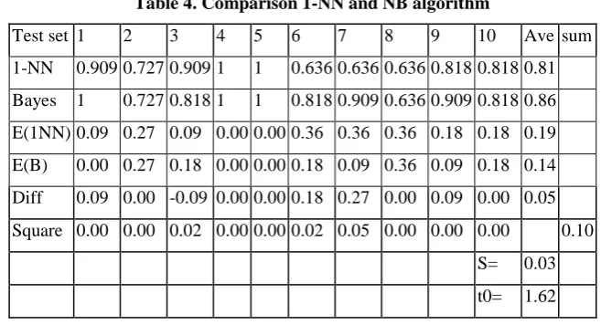
At the end, the comparison among pairs of algorithms was done. The following tables summarize the results. The first couple was 1-NN and Naive Bayes algorithm.Because t0<t.05,9= 1.833, in 90% of confidence, it can be concluded that there is no significant difference between the performance of algorithms of 1-NN and Bayes (Table 4.)
Table 4. Comparison 1-NN and NB algorithm
Test set 1 2 3 4 5 6 7 8 9 10 Ave sum 1-NN 0.909 0.727 0.909 1 1 0.636 0.636 0.636 0.818 0.818 0.81 Bayes 1 0.727 0.818 1 1 0.818 0.909 0.636 0.909 0.818 0.86 E(1NN) 0.09 0.27 0.09 0.00 0.00 0.36 0.36 0.36 0.18 0.18 0.19 E(B) 0.00 0.27 0.18 0.00 0.00 0.18 0.09 0.36 0.09 0.18 0.14 Diff 0.09 0.00 -0.09 0.00 0.00 0.18 0.27 0.00 0.09 0.00 0.05 Square 0.00 0.00 0.02 0.00 0.00 0.02 0.05 0.00 0.00 0.00 0.10
S= 0.03 t0= 1.62
Secondly, pair of K-NN and 1-NN was compared. It was found that t0>t.05,9=1.833, so, in 90% of confidence, it can be concluded that there is significant difference between the performance of algorithms of 1-NN and 3-NN (Table 5.). So, it can be said that 1-NN is better than 3-NN.
Table 5. Comparison K-NN and 1-NN algorithm
S= 0.03 t0= 1.91
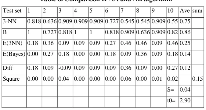
Third pair was K-NN and Naive Bayes (Table 6.). It was found that t0>t.01, 9= 2.821, and in 98% of confidence, it was concluded that there is significant difference between the performance of algorithms of 3-NN and Naive Bayes. It can be concluded that Naive Bayes algorithm performs better than 3-NN or k-NN.
Table 6. Comparison K-NN and NB algorithm
Test set 1 2 3 4 5 6 7 8 9 10 Ave sum 3-NN 0.818 0.636 0.909 0.909 0.909 0.727 0.545 0.545 0.909 0.55 0.75 B 1 0.727 0.818 1 1 0.818 0.909 0.636 0.909 0.82 0.86 E(3NN) 0.18 0.36 0.09 0.09 0.09 0.27 0.46 0.46 0.09 0.46 0.25 E(Bayes) 0.00 0.27 0.18 0.00 0.00 0.18 0.09 0.36 0.09 0.18 0.14 Diff 0.18 0.09 -0.09 0.09 0.09 0.09 0.36 0.09 0.00 0.27 0.12 Square 0.00 0.00 0.04 0.00 0.00 0.00 0.06 0.00 0.01 0.02 0.15
S= 0.04 t0= 2.90
Finally, it is obvious that performance of the algorithms changes after inserting two pairs of random and conditionally dependent features. There are no significant changes in Naive Bayes algorithms, but for K-NN, the performance decreases for about 5% after inserting two pairs of random and conditionally dependent features. The performance comparison of the two types of machine learning algorithms shows that the best solution is to use 1-NN. NB could be also used since there is no significant difference between 1-NN and NB classifier. The recommendation is to use k-NN after injecting randomness and conditional dependence in spite of decreased performance since they perform better generalization.
REFERENCES
[1] S. Deleawe, et al., Predicting Air Quality in Smart Environments, J Ambient Intell Smart Environ. 2010; 2(2): 145–152
[2] S.L. Ting, et al.,Is Naïve Bayes a Good Classifier for Document Classification?, International Journal of Software Engineering and Its Applications Vol. 5, No. 3, July, 2011
[3] D. Soria, et al.,A „non-parametric‟ version of the naive Bayes classifier, Knowledge-Based Systems, Elsevier, Vol.24, Issue 6, 2011, pages 775-784.
[4] Y. Zhao, et al. Comparison of Three Classification Algorithms for Predicting pm2.5 in Hong Kong Rural Area, Journal of Asian Scientific Research, 2013, 3(7):715-728
[5] E. G. Dragomir, Air Quality Index Prediction using K-Nearest Neighbor Technique, BULETINUL Universităţii Petrol – Gaze din Ploieşti, Vol. LXII No. 1/2010, pages 103 – 108.
[7] M. N. Murty, et al. Nearest Neighbour Based Classifiers, Springer‟s Pattern Recognition,Universities Press (India) Pvt. Ltd. 2011, pp 48-85
[8] Y. Song et al., IKNN: Informative K-Nearest Neighbor Pattern Classification, Department of Computer Science and Engineering, The Pennsylvania State University, PA, 2006