749 | P a g e
APPLICATION OF GA, PSO AND PSO-BFGS FOR
THE INVERSE ESTIMATION PROBLEM
Vishweshwara P S
1, Gnanasekaran N
2, Arun M
31,2,3
Department of Mechanical Engineering, National Institute of Technology Karnataka, Surathkal,
Srinivasnagar P.O., Mangalore, 575025, Karnataka, (India)
ABSTRACT
This paper deals with the estimation of unknown parameter using evolutionary algorithms such as Genetic
Algorithm (GA) and Particle Swarm Optimization (PSO). A hybrid algorithm is also proposed with the
combination of PSO and Broyden Fletcher Goldfarb Shanno Algorithm (BFGS). These algorithms are not
only used as optimization techniques but also applied for the estimation of unknown parameters or function
appearing in the mathematical model. Initially, the proposed evolutionary algorithms are validated with the
available benchmarks in literature. A mathematical model that represents a lumped system in heat transfer is
considered to be the forward solution. An inverse problem is proposed to estimate the unknown parameters
appearing in the forward model. In order to generate measurement data, the temperatures obtained by solving
the forward model for the known parameters are then added with noise at different levels. The unknown
parameters appearing in the mathematical model is successfully estimated using these algorithms.
Keywords: Parameter estimation, Genetic Algorithm, Particle Swarm Optimization, BFGS, Evolutionary algorithms.
I. INTRODUCTION
Evolutionary algorithms are most widely used in finding the unknown parameters using optimization concepts.
Several popularly used evolutionary algorithms are Genetic Algorithm, Particle Swarm Optimization, Bacterial
Foraging Optimization, Ant Colony Optimization, etc.,. The evolution of these new methods is based on
analysing the nature and relating their physics with mathematical theories. However, to make use of these
algorithms in solving heat transfer problems is quite challenging task as the conventional numerical methods are
popularly used to solve such problems. Several work has been attempted in the recent from past to retrieve the
unknown parametersusing deterministic methods like Steepest descent method, Levenberg method, Conjugate
Gradient Method, BFGS method etc.,. A comprehensive discussion about the deterministic and the stochastic
methods are available in [1].Many a times, deterministic methods fail to attain global minima/maxima if the
initial guess is close to the local minima/maxima. Hence, it is better to use evolutionary algorithm to overcome
such problems. Partridge and Wrobel used GA for bio heat transfer problems and proved that GA is an effective
750 | P a g e
for variety of weld geometry. Panda and Das estimated the geometrical configurations of a porous fin using GAas an inverse method [4]. The combination of deterministic method and evolutionary algorithms has been used
to determine the heat transfer coefficient for continuous casting process using PSO and Gaussian Kernel
function [5]. Nusselt number correlation has been developed using PSO for thin fins in narrow cavity based on
temperature measurement [6]. The application of PSO has also been reported for radiation problem [7].Dora
and Tortorellit solved the inverse heat conduction problem and compared the results with numerical solutions
[8]. A comparison study based on the modified BFGS with PSO resulted in obtaining quality resultsfor
solvingstandard benchmark problems [9]. Victoire and Jeyakumar applied PSO-BFGS for different economic
dispatch problem [10].The application of evolutionary algorithm was also found in field of biomechanics where
Jaco et al, compared PSO algorithm with GA, BFGS and SQP for identifying the human muscle movements
[11]. The work on hybrid PSO algorithm was effectively employed in other engineering applications too [12,
13].
II. PROBLEM STATEMENT FOR A LUMPED SYSTEM
In the present work, the mathematical model represents a lumped system having high thermal conductivity and
is subjected to natural convection heat transfer. The initial temperature of the high thermal conductivity material
is 100°C and the material is kept in quiescent air at 30°C. Fig. 1 shows the schematic representation of the
present model. Let be the surface area in m2, is the mass in kg, is the specific heat in J/kgK, τ is the
time constant and h is the convectiveheat transfer coefficient in W/m2K. The thermo-physical properties and the
experimental temperature distribution are chosen from [14]. Then, the governing equation becomes,
(1)
(2)
(3)
(4)
751 | P a g e
Table 1. Temperature time history of the system. [14]
S. No Time,s Temperature,
1 10 93.3
2 30 82.2
3 60 68.1
4 90 57.9
5 130 49.2
6 180 41.4
7 250 36.3
8 300 32.9
The main aim of the present work is to estimate the value of the time constant (τ) by using the temperature time
history of the system as shown in Table 1. In order to estimate the time constant, an objective function is defined
based on the least squares as shown in equation (5).
(5)
Where τ is the unknown parameter. is the pth observation from the measurements, is the temperature
values obtained by solving the equation(4).
III.GENETIC ALGORITHM
The Genetic algorithm wasdeveloped by Goldberg and Holland [15]. The basic steps in the genetic algorithm
include selection of the input parameters called population initialization, evaluation of fitness function,
reproduction, cross over, mutation and final solution. In the Initialization step, a range of input values is defined
in terms of corresponding binary values. These values are called chromosomes. A range of input is referred to as
set of chromosomes.
Example: For a value of 1500, corresponding binary number is
Guess number: 1500
Binary: 10111011100
Each individual (0 or 1) is referred to as chromosomewhich contains certain number of digits called genes. In
the above example, the number of genes is 11. Fitness function is evaluated for each of these input values. The
752 | P a g e
IV.PSO ALGORITHM
In 1995, Kennedy and Eberhart developed Particle Swarm Optimization (PSO) as a robust technique which can
be implemented to various inverse problems [16]. In comparison with the existing biological algorithms, PSO
uses lesser parameters to solve the objective function. In a search space of N dimension with M particles moving
in a swarm, the position and the velocity vectors of the ith particle are given by Xi=(xi1,xi2,....,xiM) and
Vi=(vi1,vi2,...,viN). In every generation, the addition of displacement to the present location will give a new
position which is given by,
(6)
The corresponding updated velocity from the previous velocity of the each particle in the direction of
and is given as,
(7)
Particles contain particle best according to fitness value that contains the information of their previous position.
. The best position of the swarm particle isidentified as global
best . The second term in Equation (7) is called as cognition part associated with
cognition learning coefficient ,which can control the movement of the particle. The third term is the social
component associated with , that makes the particles to decided next position. and are the random
numbers whose value lie from 0 to 1. The sum of the values of and should be lesser or equal to 4. Variable
w is the inertia weighting function which has an important role in controlling exploration capacities of the
swarms. The value of w lies between 0 and 1. For the present work, variable value is expressed as
(8)
V.PSO-BFGS ALGORITHM
PSO sometimes suffer premature convergence [17]. This can be overcome by combining PSO with BFGS
method. The method improves the particles to search locally with a better solution. For nonlinear optimization,
the use of BFGS method is very efficient as its performance is found to be more accurate compared to other
optimization algorithms. The procedure for BFGS is explained as below [18].
Step 1: Set the value of initial point and convergence criterion ε>0.
Step 2: Initialize a Hessian matrix , calculate the gradient
Hessian matrix of the Lagrangian function is evaluated in each iteration replacing the previous Hessian
753 | P a g e
Step 3:(9)
Step 4: Set the values
(10)
(11)
The value can be computed by the below equation (12),
(12)
Step 5: If , calculation is stopped and the output is the solution. Else go to
Step 6: set and evaluate which is given by
(13)
Step 7: Set the value k to next iteration k+1 and go to step 3.
For PSO-BFGS method, after finding the global best for the current iteration using PSO [10]
Step 8: if , solve the inverse problem with BFGS algorithm using the present global best .
Step 9: Replace the value with the final solution obtained using BFGS method, else
Step 10: go to step 4.
Step 11: change the velocities and positions.
Step 12: iteration continued till the stopping criterion is reached.
VI.ESTIMATION OF THE UNKNOWN PARAMETER
The unknown parameter appearing in the mathematical model is now solved using GA, PSO and PSO-BFGS as
inverse methods. Before attempting the solution to the present inverse problem, a benchmark problem is solved
using the above mentioned evolutionary algorithms to provide a firm establishment of the ability of these
algorithms. The bench mark problem used is Rosenbrock banana function [19] which is given by Equation (14)
754 | P a g e
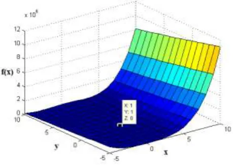
The range of is chosen between -5 and 10. The retrieved values using the mentioned algorithms aretabulated in Table 2. The minimum of the banana function lies at (1,1). The 3D plot of the Banana function is
shown in Fig.2. Fig.3 shows the evaluation of Rosenbrock function using GA, PSO and PSO-BFGS and it is
evident that the in-house code was able to predict the values of and accurately.
Fig.2. 3D representation of Banana function.
Fig.3. Minimum values of Rosenbrock banana function.
Table 2. Retrieved values of x and y using mentioned algorithms.
GA PSO PSO-BFGS
Runs x y Time,s x y Time,s X y Time,s
1 1 1 0.491 1 1 0.27 1 1 0.284
2 1 1 0.484 1 1 0.298 1 1 0.277
755 | P a g e
Fig.4. Overall representation of the work.
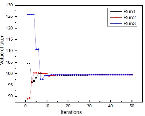
Fig.5. Retrieval of time constant for different runs using GA.
Figure 4 represents the overall representation of the present approach and Fig.5 shows the retrieval of time
constant (τ) using GA method and the solution is obtained for several trials and three such runs are reported in
Table 3 for the same range of inputs. The number of iterations is set to 50. The value of τ is randomly chosen
within the range [10 500]. The mutation rate, chromosomes number and gene number are assigned to be 0.1, 10
and 12, respectively. Each chromosome in the range assumed represents the values of τ. The difference between
Temperatures and actual temperature Ti is calculated in the objective function. The minimum, mean and
756 | P a g e
which will be considered for the future iterations. The effect of algorithm parameters like chromosome numberand gene number is also studied and the values are tabulated in Table 4 and 5 respectively.
Table 3. Estimated values for the τ using GA for several runs.
Runs τ Time,s
1 99.55 0.234
2 99.49 0.244
3 99.55 0.246
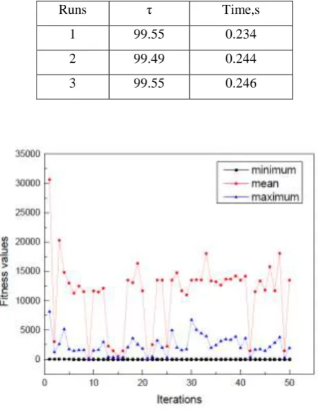
Fig.6. Fitness values of the GA.
Table 4. Effect of chromosome number on estimation using GA.
Chromosome number τ Time,s
10 99.5 0.256
20 101.89 0.27
30 99.55 0.31
Table 5. Effect of gene number on estimation using GA.
genes τ Time, s
8 102.23 0.212
757 | P a g e
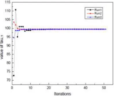
The estimation of τ is further carried out using PSO algorithm for the same range of τ value. To evaluate theobjective function, swarms, number of particles, are also initialized. In the present study, the particles represent
a range of τ. For every iteration, the particle’s previous best and the global best are updated. The values of
and are set to 1.43 and 1.43, respectively. After the evaluation of fitness function, the personal best and
global best values are updated appropriately. In the next iteration, the updated velocities and positions of each
particle are considered.The estimated values of three such runs are tabulated in Fig.7 and the values are
tabulated in Table 6. The position and velocities are generated randomly. Similar to GA, effect of number of
particles on estimation is tabulated in Table 7.
Fig.7. Retrieval of tau for different runs using PSO.
Table 6. Estimation of τ using PSO.
Runs τ Time, s
1 99.46 0.21
2 99.46 0.176
3 99.46 0.2
Table 7. Effect of particle numbers on estimation using PSO.
Particle numbers τ Time, s
10 99.46 0.21
20 99.46 0.18
30 99.46 0.21
The adaptation of hybrid method, PSO-BFGS algorithm is carried out using the same initial guess as PSO but
758 | P a g e
find the increment for new modified value of global best of the particle. Results of PSO-BFGS method areshown in Table 8for three different runs and plotted in Fig.8.
Table 8.Estimation of τ using PSO BFGS.
Runs τ Time, s
1 99.46 0.4
2 99.46 0.32
3 99.46 0.28
The computational time required for the estimation of heat flux using PSO-BFGS algorithm was observed to be
slightlymore compared to other two algorithms because it needs to find out appropriate value of α to predict the
increment of the next parameter. The effect of number of particles is also mentioned for the proposed hybrid
scheme which is shown in Table 9.
Table 9. The effect of number of particles on estimation using PSO-BFGS.
Particle numbers τ Time, s
10 99.46 0.28
20 99.46 0.3
30 99.46 0.35
759 | P a g e
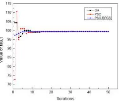
Fig.9. Comparison of estimated values of τ for different algorithms.
Figure 9 shows the comparison for the convergence of estimated τ values for mentioned algorithms. Fig.10
shows the comparison of fitness values for GA, PSO and PSO BFGS algorithms respectively. From the above
results on the estimation of time constant (τ), it can be observed that the all the three algorithms were successful in estimating τ. The study on effect of algorithms parameters like number of population, gene number for GA
showed some inconsistency in estimating the value of τ as shown in the table 4 and 5 respectively.
Fig.10. Comparison of fitness function values for different algorithms.
In case of PSO and PSO-BFGS, the estimation was consistent for all the runs. It depends on the complexity of
the problem. Generally, for any evolutionary algorithm, the increase in the population size or particle size will
increase the computational cost and there will be faster convergence of the solution as it provides a large search
space for the estimation process [17, 20].The results obtained by all the mentioned algorithms were comparable
and with the promising results obtained from PSO-BFGS one can apply this hybrid technique for complex
760 | P a g e
VII.CONCLUSION
In this paper study, the solution of a lumped system in heat transfer is solved using evolutionary algorithms GA,
PSO and PSO-BFGS. The in-house code has been verified with the benchmark problems. The inverse
estimation is accomplished for the measurement data available in literature. In order to solve the time constant
value, the objective function is framed according to least squares method. Thus, results obtained with all the
algorithms show good estimates in the field of parameter estimation. Later, itwas concluded that the
PSO-BFGS,a new hybrid optimization algorithm, can effectively be used to solve the heat transfer problems. All the
three algorithms were found effective in parameter estimation hence provides a great hope in estimating the
unknown parameters in the field of heat transfer.
REFERENCES
[1] M.J. Colaço, H.R.B. Orlande,G. S. Dulikravich, Inverse and Optimization Problems in Heat Transfer,
Journal of the Brazilian Society of Mechanical Science and Engineering, 28 (1),2006, 1-24 .
[2] P.W. Partridge, L.C. Wrobel, An inverse geometry problem for the localisation of skin tumours by thermal
analysis, Engineering Analysis with Boundary Elements, 31, 2007, 803–811.
[3] S. Bag , A. De, T. DebRoy, A Genetic Algorithm-Assisted Inverse Convective Heat Transfer Model for
Tailoring Weld Geometry, Materials and Manufacturing Processes, 24, 200, 384–397.
[4] S. Panda, R. Das, Inverse analysis of a radial porous fin using genetic algorithm, Eighth International
Conference on Contemporary Computing (IC3), 2015, DOI: 10.1109/IC3.2015.7346673.
[5] X.C. Luo, Q. Xie, Y. Wang, C. Yang, Estimation of heat transfer coefficients in continuous casting under
large disturbance by Gaussian kernel particle swarm optimization method, International Journal of Heat and
Mass Transfer, 111, 2017, 1087–1097.
[6] A. Azimifar, S. Payan, Optimization of characteristics of an array of thin fins using PSO algorithm in
confined cavities heated from a side with free convection, Applied Thermal Engineering, 110,2017, 1371–
1388.
[7] H. Qi, D.L. Wang, S.G. Wang, L.M. Ruan, Inverse transient radiation analysis in one-dimensional
non-homogeneous participating slabs using particle swarm optimization algorithms, Journal of Quantitative
Spectroscopy &Radiative Transfer, 112, 2011, 2507-2519.
[8] G.A. Dora, D. Tortorellit, Transient inverse heat conduction problem solutions via Newton’s method,
International Journal of Heat and Mass Transfer
,
40 (17), 2010, 4115-4127.[9] S. Li, M. Tan, I. W. Tsang, J. Tin-Yau Kwok, A Hybrid PSO-BFGS Strategy for Global Optimization of
Multimodal Functions, IEEE Transactions On Systems, Man, And Cybernetics-Part B: Cybernetics,( 41),
no.4, 2011.
[10]T.A.A. Victoire, A.E.Jeyakumar, Hybrid PSO–SQP for economic dispatch with valve-point effect, Electric
761 | P a g e
[11] J.F. Schutte, B.I. Koh, J.A. Reinbolt, R.T. Haftka, A.D. George, B.J. Fregly, Evaluation of a ParticleSwarm Algorithm For Biomechanical Optimization, Journal of Biomechanical Engineering, 127, 2005,
465-474.
[12] G. Wu, D. Qiu, Y. Yu, W. Pedrycz, M. Ma, H. Li, Superior solution guided particle swarm optimization
combined with local search techniques,
Expert Systems with Applications, 41(16),
2014, 7536-7548.[13] M.G. Miab, A.F. Farahani, R.F. Dana, C. Lucas,An efficient hybrid swarm intelligence-gradient
optimization method for complex time green’s functions of multilayer media, Progress In Electromagnetics
Research, 77 2007, 181–192.
[14] C.Balaji, Essentials of Thermal System Design and Optimization (Ane Book Pvt. Ltd., New Dehli, 2011).
[15] D.E. Goldberg, J.H.Holland, Genetic algorithms and machine learning. Machine Learning, 3(2), 1988, 95–
99.
[16] J. Kennedy, R.C. Eberhart, Particle swarm optimization, Proc. IEEE Int. Conf. on Neural Networks,1995
1942–1948.
[17] S. Vakili, M.S. Gadala, Effectiveness and Efficiency of Particle Swarm Optimization Technique in Inverse
Heat Conduction Analysis, Numerical Heat Transfer, part B: Fundamentals, 56, 2009, 119–141.
[18]H.Li, J.Lei, Q. Liu, An inversion approach for the inverse heat conduction problems, International Journal
of Heat and Mass Transfer 55, 2012, 4442–4452.
[19]H.H. Rosenbrock, An Automatic Method for Finding the Greatest or Least Value of a Function, 3 (3), 1960,
175-184.
[20] F.B. Liu, A modified genetic algorithm for solving the inverse heat transfer problem of estimating plan
![Table 1. Temperature time history of the system. [14]](https://thumb-us.123doks.com/thumbv2/123dok_us/7783696.1286810/3.595.199.398.143.310/table-temperature-time-history.webp)