Set-Membership Quaternion Normalized
LMS Algorithm
Hamid Reza Moradi and Akram Zardadi
Abstract
In this paper, we propose the set-membership quaternion normalized least-mean-square (SM-QNLMS) algo-rithm. For this purpose, first, we review the quaternion least-mean-square (QLMS) algorithm, then go into the quaternion normalized least-mean-square (QNLMS) algorithm. By having the QNLMS algorithm, we propose the SM-QNLMS algorithm in order to reduce the update rate of the QNLMS algorithm and avoid updating the system parameters when there is not enough innovation in upcoming data. Moreover, the SM-QNLMS algorithm, thanks to the time-varying step-size, has higher convergence rate as compared to the QNLMS algorithm. Finally, the proposed algorithm is utilized in wind profile prediction and quaternionic adaptive beamforming. The simulation results demonstrate that the SM-QNLMS algorithm outperforms the QNLMS algorithm and it has higher convergence speed and lower update rate.
Index Terms
Adaptive filtering, set-membership filtering, quaternion, SM-QNLMS, wind profile prediction, quaternionic adaptive beamforming.
I. INTRODUCTION
T
HE quaternions are a number system that extends the complex numbers. Initially, they were intro-duced by William Rowan Hamilton in 1843 [1]. They have many applications to multivariate signal processing problems, such as wind profile prediction [2]–[4], color image processing [5], [6], and adaptive beamforming [4], [7], [8]. A broad family of quaternion based algorithms have been proposed in adaptive filtering literatures [4], [9]–[12].The quaternion domain generalizes the complex domain and gives us a useful way to process 3- and 4-dimensional signals. In recent years, many quaternion based adaptive filtering algorithms have been introduced, and they take advantage of the fact that the quaternion domain is a division algebra and it has suitable data representation [13], [14]. Hence, the quaternion algorithms permit a coupling between the components of 3- and 4-dimensional processes. Furthermore, the quaternion-valued algorithm brings better performance in comparison with the real-valued algorithms, since it accounts for the coupling of the wind measurements and can be boosted to exploit the augmented quaternion statistics [15]. As a result, as compared to the real-valued algorithms in R3 and R4, they present better stability and more degrees of freedom in the control of the adaptation process.
In this work, we assume an effective approach in order to reduce the computational resources of an adaptive filter by employing set-membership filtering (SMF) technique [16]–[18]. For real numbers, the set-membership normalized least-mean-square (SM-NLMS) [16], [18], [19] and the set-membership affine projection (SM-AP) [18], [20], [21] algorithms have already been proposed. There are many variants of the set-membership algorithms and their applications in adaptive filtering literatures [22]–[26]. Moreover, the set-membership quaternion affine projection algorithm has already been introduced in [4]. Here, by generalizing the SM-NLMS algorithm, we want to introduce the set-membership quaternion normalized
(H. R. Moradi) YOUNG RESEARCHERS AND ELITE CLUB, MASHHAD BRANCH, ISLAMIC AZAD UNIVERSITY, MASHHAD, IRAN.
E-mail address: [email protected].
(A. Zardadi) DEPARTMENT OF MATHEMATICS, PAYAME NOOR UNIVERSITY (PNU), P.O. Box, 19395-4697, TEHRAN, IRAN. E-mail address: [email protected].
2010 Mathematics Subject Classification: 68T05, 68Q32, 68W27.
least-mean-square (SM-QNLMS) algorithm to operate with the quaternion numbers. The product of quaternion numbers is not commutative, and the proposed algorithm gets around this drawback.
Ultimately, we apply the SM-QNLMS algorithm to predicting the wind profile and compare their competitive performance with the quaternion least-mean-square (QLMS) and the quaternion normalized least-mean-square (QNLMS) algorithms. Moreover, we study the quaternion adaptive beamforming as an application of the quaternion-valued algorithms. In this manner, we will reduce the number of involved sensors in the adaptation mechanism. As a result, we can decrease the computational complexity and the energy consumption of the system. As demonstrated in numerical results, we recognize that the SM-QNLMS algorithm has higher convergence rate and lower update rate as compared to the QLMS and the QNLMS algorithms.
This paper is organized as follows. A short introduction to quaternions is provided in Section II. Section III briefly reviews the concept of SMF, but instead of real numbers, we utilize quaternions. Section IV reviews the QLMS algorithm, and the SM-QNLMS algorithm is derived in Section V. Simulations and numerical results are provided in Section VI, and Section VII draws the conclusions.
Notations: Scalars are denoted by lower case letters. Vectors (matrices) are represented by lowercase (uppercase) boldface letters. The quaternion number system is represented byH. At iteration k, the weight vector and the input vector are denoted by w(k),x(k)∈HN+1, respectively, where N is the adaptive filter
order. For a given iteration k, the error signal is defined as e(k), d(k)−wH(k)x(k), where d(k)∈ H
is the desired signal and (·)H stands for the vector and matrix hermitian.
II. QUATERNIONS
The quaternion number system is a non-commutative extension of complex numbers, represented by
H. A quaternion number q ∈H is described by [1]
q=qa+qbı+qc+qdκ, (1)
where qa, qb, qc, and qdare real numbers. The real component of q is qa, whileqb, qc, andqd are its three
imaginary components. The orthogonal unit imaginary axis vectors ı, , and κ satisfy in the following rules
ı=κ κ=ı κı=,
ı2 =2 =κ2 =ıκ=−1. (2) Note that the quaternion multiplication is a non-commutative operator; we haveı=−κ6=ıfor example. The element 1 is the identity element of H. The conjugate of a quaternionq, represented byq∗, is defined
as
q∗ =qa−qbı−qc−qdκ, (3)
and the norm |q| is expressed by
|q|=√qq∗ =qq2
a+qb2+qc2+qd2. (4)
The inverse of q is proposed as
q−1 = q
∗
|q|2. (5)
Note that q can be reformulated into the Cayley-Dickson [7] form through
q= (qa+qc)
| {z }
z1
+ı(qb+qd)
| {z }
z2
, (6)
III. SET-MEMBERSHIP FILTERING (SMF) INH
The aim of the SMF is to obtain w such that the magnitude of the output estimation error is upper
bounded by a predetermined positive value γ. We can change the value of γ with the specific application. If the value of γ is properly adopted, there are many valid estimates for w. Assume thatS denotes the set
of all possible input-desired data pairs (x, d) of interest and denote by Θ the set of all vectors w whose
magnitudes of their output estimation errors are upper bounded by γ whenever (x, d) ∈ S. The set Θ is
called feasibility set and is introduced by
Θ, \ (x,d)∈S
{w∈HN+1 :|d−wHx| ≤γ}, (7)
Let’s define the constraint set H(k) containing all vectors w such that the magnitude of their output
estimation errors at time instant k are upper bounded by γ,
H(k),{w∈HN+1 :|d(k)−wHx(k)| ≤γ}. (8)
Then the membership set ψ(k) is introduced by
ψ(k),
k
\
i=0
H(i). (9)
The membership set will contain Θand will coincide withΘif all data pairs in S are traversed up to time instant k. Due to difficulties to calculate ψ(k), adaptive approaches are needed [16]. The simplest method is to calculate a point estimate utilizing, for example, the information provided by the constraint set H(k)
as in the set-membership normalized least-mean-square algorithm [16], or several preceding constraint sets as in the set-membership affine projection algorithm [20].
IV. THE QUATERNION NORMALIZED LMS ALGORITHM
In this section, we review the quaternion normalized LMS (QNLMS) algorithm. For this purpose, first, we remind the quaternion LMS (QLMS) algorithm. The QLMS algorithm for quaternion signals, which usually appear in image signal processing and multidimensional signal processing applications, is derived in [2]. The updating equation for the QLMS algorithm is described by
w(k+ 1) =w(k) +µe∗(k)x(k). (10)
The parameter µin the equation above is the step-size, and it should be selected small enough to guarantee the convergence of the algorithm. In general, the QNLMS algorithm presents better performance than the QLMS algorithm in many applications. The update equation of the QNLMS algorithm can be characterized as
w(k+ 1) =w(k) +µ e
∗(k)x(k)
xH(k)x(k) +δ =
w(k) +µ e
∗(k)x(k)
kx(k)k2+δ, (11)
where kx(k)k2+δ is the normalizing term and δ ∈ R+ is a small positive constant introduced to avoid
V. THE SET-MEMBERSHIP QUATERNION NORMALIZED LMS ALGORITHM
The set-membership QNLMS (SM-QNLMS) algorithm has a structure analogous to the QNLMS algorithm. The fundamental idea of the SM-QNLMS algorithm is to implement an evaluation to check if the previous weight vector w(k) belongs to the constraint set H(k). If the norm of the output estimation
error signal e(k) is greater than the predetermined positive value γ, the new weight vectorw(k+ 1) will
be updated to the closest boundary of the constraint set H(k) at a minimum distance. In other words, the objective function of the SM-QNLMS algorithm is given by
min kw(k+ 1)−w(k)k2
subject to
w(k+ 1) ∈ H(k). (12)
The updating procedure is obtained by implementing an orthogonal projection of the previous weight vector onto the closest boundary of H(k).
To obtain the recursion rule of the SM-QNLMS algorithm, assume that the a priori error e(k) is given by
e(k) = d(k)−wH(k)x(k), (13)
and consider the update equation of the QNLMS algorithm with the variable step-size µ(k) as follows
w(k+ 1) =w(k) + µ(k) xH(k)x(k) +δe
∗(k)x(k). (14)
In order to attain the update equation of the SM-QNLMS algorithm, we require to adopt µ(k) suitably such that it satisfies the desired set-membership updating. Indeed, the update must happen if
|e(k)|=|d(k)−wH(k)x(k)|> γ (15)
and the norm of the a posteriori error must be given by
|ε(k)|=|d(k)−wH(k+ 1)x(k)|=γ
=|d(k)−wH(k)x(k)− µ(k)
xH(k)x(k) +δe(k)
xH(k)x(k)|
=|e(k)− µ(k)
xH(k)x(k) +δe(k)
xH(k)x(k)|, (16)
where |ε(k)| =γ because w(k) is updated to the closest boundary of H(k). The parameter δ is a small
constant since it is responsible for regularization to avoid numerical problems, thus it can be neglected leading to
|ε(k)|=|e(k)(1−µ(k))|=γ (17)
⇒|1−µ(k)|= γ
|e(k)| >0 (18)
⇒1−µ(k) = γ
|e(k)| (19)
⇒µ(k) = 1− γ
|e(k)|. (20)
Our purpose is to implement update when |e(k)|> γ, thus the variable step-size is given by µ(k) =
1− |e(γk)| if |e(k)|> γ,
0 otherwise. (21)
Finally, the SM-QNLMS algorithm is summarized in Table I. As a rule of thumb, the value ofγ is adopted about p5σ2
TABLE I
SET-MEMBERSHIP QUATERNIONNLMSALGORITHM
SM-QNLMS Algorithm
Initialization
w(0) = [0 · · · 0]T
chooseγ around√5σ2
n
choose small positive constantδ Do fork≥0
e(k) =d(k)−wH(k)x(k)
µ(k) =
1− γ
|e(k)| if|e(k)|> γ,
0 otherwise.
w(k+ 1) =w(k) + µ(k)
xH(k)x(k)+δe
∗(k)
x(k)
end
VI. SIMULATIONS
In this section, we utilize the QLMS, the QNLMS, and the SM-QNLMS algorithms in two scenarios. In Scenario 1, we use these algorithms in wind profile prediction and, in Scenario 2, we implement quaternionic adaptive beamforming by these algorithms.
A. Scenario 1
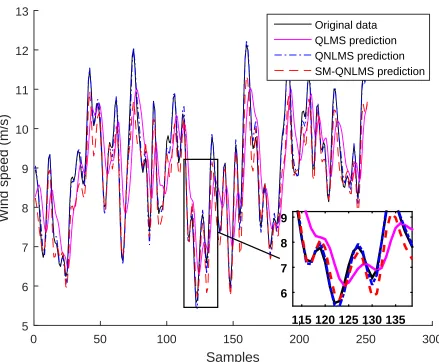
In this scenario, the QLMS, the QNLMS, and the SM-QNLMS algorithms are applied to anemometer readings provided by Google’s RE<C Initiative [28]. The wind speed recorded on May 25, 2011, is utilized for the algorithms comparisons. The step-size, µ, is adopted as 10−8 and 0.9 for the QLMS and
the QNLMS algorithms, respectively. The value of γ is chosen as 5. The filter order is 7, i.e., w(k)
contains 8 coefficients, and the prediction step is selected equal to 1. All algorithms are initialized with the zero vector.
Figure 1 shows the predicted results using the QLMS, the QNLMS, and the SM-QNLMS algorithms. We can observe that the QLMS algorithm, the solid magenta curve, cannot track the wind speed, the solid black curve, as well as the QNLMS algorithm, the dash-dotted blue curve, and the SM-QNLMS algorithm, the dashed red curve. As can be seen, the SM-QNLMS algorithm is tracking the wind speed as well as the QNLMS algorithm; however, the SM-QNLMS algorithm has lower update rate and avoid updating the filter coefficients when there is no innovation in upcoming data. Indeed, the update rate of the SM-QNLMS algorithm is 17.9%, whereas the update rate of the QNLMS algorithm is 100%. Therefore, the SM-QNLMS algorithm has a significantly higher computational efficiency as compared to the QNLMS algorithm, and this algorithm outperforms the QLMS and the QNLMS algorithms.
B. Scenario 2
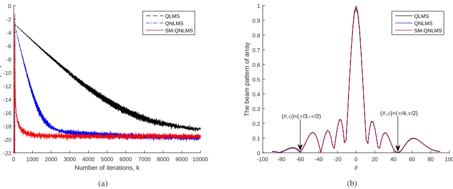
One of the most important applications of the quaternion-based adaptive algorithms is in quaternionic adaptive beamforming. By utilizing the crossed-dipole array and quaternions, we can reduce the number of engaged sensors in the adaptive beamforming process. Hence, the computational complexity and the energy consumption of the system will decrease without losing the quality of the performance [8], [17], [29]–[31].
In this scenario, we perform the quaternionic adaptive beamforming [3], [17] utilizing the QLMS, the QNLMS, and the SM-QNLMS algorithms. We assume a sensor array with 10 crossed-dipoles and half-wavelength spacing. The step size, µ, for the QLMS and the QNLMS algorithms are 4×10⁻⁵ and 0.009,
respectively. A desired signal with 20 dB SNR (σ2
Samples
0 50 100 150 200 250 300
Wind speed (m/s)
5 6 7 8 9 10 11 12 13
Original data QLMS prediction QNLMS prediction SM-QNLMS prediction
115 120 125 130 135 6
7 8 9
Fig. 1. Predicted results from the QLMS, the QNLMS, and the SM-QNLMS algorithms.
and two interfering signals with signal-to-interference ratio (SIR) of -10 dB arrive from (θ, φ) = (π
4,
π
2)
and (θ, φ) = (π
3,−
π
2), respectively. All the signals have the same polarization of (γ, η) = (0,0), and γ is
set to be p2σ2
n.
The learning curves of the QLMS, the QNLMS, and the SM-QNLMS algorithms over 100 independent runs are depicted in Figure 2(a). The average number of updates performed by the SM-QNLMS algorithm is 1425 in a total of 10000 iterations, i.e., 14.25%. As can be seen, the SM-QNLMS algorithm converges faster while having a lower number of updates as compared to the QNLMS algorithm. Indeed, the SM-QNLMS algorithm not only reduces the update rate but also increases the convergence rate in comparison with the QNLMS algorithm. Furthermore, as can be seen, the QLMS algorithm has lower MSE and extremely low convergence speed as compared to the QNLMS and the SM-QNLMS algorithms.
The response of a beamformer to the impinging signals as a function of θ is called beam pattern and is defined as B(θ) =wHs(θ), where s(θ) is the steering vector. The magnitude of beam pattern explains
the variation of a beamformer concerning the signal arriving from different Direction of Arrival (DOA) angles. Figure 2(b) presents the magnitude of the beam pattern of the QLMS, the QNLMS, and the SM-QNLMS algorithms with θ = 0. In Figure 2(b), the positive values of θ show the value range θ ∈ [0,π2]
for φ = π
2 and the negative values, θ ∈ [−
π
2,0], indicate the same range of θ ∈ [0,
π
2] but φ =−
π
2. We
Number of iterations, k
0 1000 2000 3000 4000 5000 6000 7000 8000 9000 10000
MSE [dB]
-22 -20 -18 -16 -14 -12 -10 -8 -6 -4 -2 0
QLMS QNLMS SM-QNLMS
(a)
θ
-100 -80 -60 -40 -20 0 20 40 60 80 100
The beam pattern of array
0 0.1 0.2 0.3 0.4 0.5 0.6 0.7 0.8 0.9 1
QLMS QNLMS SM-QNLMS
(θ,φ)=(π/3,-π/2) (θ,φ)=(π/4,π/2)
(b)
Fig. 2. (a) The MSE learning curves of the QLMS, the QNLMS, and the SM-QNLMS algorithms; (b) Beam patterns of the QLMS, the QNLMS, and the SM-QNLMS algorithms when DOA of the desired signal is(θ, φ) = (0,π
2).
TABLE II
THEOSDRAND THEOSIRFOR THEQLMS,THEQNLMS,AND THESM-QNLMSALGORITHMS
Algorithms QLMS QNLMS SM-QNLMS
OSDR (dB) -1.651 -1.508 -0.026
OSIR (dB) -11.702 -11.564 -10.074
The output signal to desired plus noise ratio (OSDR) and the output signal to interference plus noise ratio (OSIR) for the QLMS, the QNLMS, and the SM-QNLMS algorithms are presented in Table II. The OSDR is attained by computing the power of the output signal and the total power of desired plus one-third of the noise signal, and then we compute the ratio between these two values. Also, the OSIR is achieved by calculating the power of the output signal and the total power of interference plus one-third of the noise signal, and then we find the ratio between the two. We can observe that the best results are attained by the SM-QNLMS algorithm.
VII. CONCLUSIONS
In this paper, we have reviewed some properties of quaternion numbers, and we have discussed the set-membership filtering strategy in the systems of quaternion numbers. Also, we have studied the QLMS algorithm, and by normalizing this algorithm, we have represented the QNLMS algorithm. Then we have proposed the SM-QNLMS algorithm aiming at reducing the update rate of the QNLMS algorithm. Finally, we have examined these algorithms in wind profile prediction and quaternionic adaptive beamforming. As indicated by the numerical results, the SM-QNLMS algorithm not only has higher computational efficiency as compared to the QNLMS algorithm but also obtains significant higher convergence speed.
REFERENCES
[1] W.R. Hamilton, “On quaternions, or a new system of imaginaries in algebra”, Philosophical Magazine, v. 25, n. 3, pp. 489–495, 1844. [2] Q. Barth´elemy, A. Larue, and J.I. Mars, “About QLMS derivations”, IEEE Signal Processing Letters, v. 21, n. 2, pp. 240–243, February
2014.
[4] H. Yazdanpanah and P.S.R. Diniz, “New trinion and quaternion set-membership affine projection algorithms”, IEEE Transactions on
Circuits and Systems II: Express Briefs, v. 64, n. 2, pp. 216–220, February 2017.
[5] S.C. Pei, J.H. Chang, and J.J. Ding, “Commutative reduced biquaternions and their Fourier transform for signal and image processing applications”, IEEE Transactions on Signal Processing, v. 52, n. 7, pp. 2012–2031, July 2004.
[6] L.Q. Guo, M. Zhu, and X.H. Ge, “Reduced biquaternion canonical transform, convolution and correlation”, Signal Processing, v. 91, n. 8, pp. 2147–2153, August 2011.
[7] X.R. Zhang, W. Liu, Y.G. Xu, et al. “Quaternion-valued robust adaptive beamformer for electromagnetic vector-sensor arrays with worst-case constraint”, Signal Processing, v. 104, pp. 274–283, November 2014.
[8] M. Jiang, “Quaternion-valued adaptive signal processing and its application to adaptive beamforming and wind profile prediction”,
University of Sheffield, D.Sc. Thesis, 2016.
[9] B.C. Ujang, C.C. Took, and D.P. Mandic, “Quaternion-valued nonlinear adaptive filtering”, IEEE Transactions on Neural Networks, v. 22, n. 8, pp. 1193–1206, August 2011.
[10] C.C. Took and D.P. Mandic, “The quaternion LMS algorithm for adaptive filtering of hypercomplex processes”, IEEE Transactions on
Signal Processing, v. 57, n. 4, pp. 1316–1327, April 2009.
[11] C.C. Took, D.P. Mandic, and J. Benesty, “Study of the quaternion LMS and four-channel LMS algorithms”. In: IEEE International
Conference on Acoustics, Speech and Signal Processing (ICASSP), Taipei, Taiwan, pp. 3109-3112, April 2009.
[12] F.G.A. Neto and V.H. Nascimento, “A novel reduced-complexity widely linear QLMS algorithm”. In: IEEE Statistical Signal Processing
Workshop (SSP), Nice, France, pp. 81-84, June 2011.
[13] S.-C. Pei and C.-M. Cheng, “Color image processing by using binary quaternion-moment-preserving thresholding technique”, IEEE
Transactions on Image Processing, v. 8, n. 5, pp. 614–628, May 1999.
[14] N. Le Bihan and S.J. Sangwine, “Quaternion principal component analysis of color images”. In: International Conference on Image
Processing (ICIP), Barcelona, Spain, pp. I-809-12 vol.1, September 2003.
[15] C.C. Took, G. Strbac, K. Aihara, and D.P. Mandic, “Quaternion-valued short term joint forecasting of three-dimensional wind and atmospheric parameters”, Renewable Energy, v. 36, n. 6, pp. 1754–1760, June 2011.
[16] S. Gollamudi, S. Nagaraj, S. Kapoor, and Y.-F. Huang, “Set-membership filtering and a set-membership normalized LMS algorithm with an adaptive step size,” IEEE Signal Processing Letters, vol. 5, no. 5, pp. 111–114, May 1998.
[17] H. Yazdanpanah, “On data-selective learning”, Federal University of Rio de Janeiro, D.Sc. Thesis, 2018.
[18] P.S.R. Diniz, “Adaptive Filtering: Algorithms and Practical Implementation”, Springer, 4th edition, New York, USA, 2013.
[19] H. Yazdanpanah, M.V.S. Lima, and P.S.R. Diniz, “On the robustness of the set-membership NLMS algorithm”. In: 9th IEEE Sensor
Array and Multichannel Signal Processing Workshop (SAM), Rio de Janeiro, Brazil, pp. 1-5, July 2016.
[20] S. Werner and P.S.R. Diniz, “Set-membership affine projection algorithm,” IEEE Signal Processing Letters, vol. 8, no. 8, pp. 231–235, August 2001.
[21] H. Yazdanpanah, M.V.S. Lima, and P.S.R. Diniz, “On the robustness of set-membership adaptive filtering algorithms”, EURASIP Journal
on Advances in Signal Processing, v. 72, pp. 1–12, December 2017.
[22] J.F. Galdino, J.A. Apolin´ario, Jr., and M.L.R. de Campos, “A set-membership NLMS algorithm with time-varying error bound”. In:
IEEE International Symposium on Circuits and Systems (ISCAS), Island of Kos, Greece, pp. 277-280, May 2006.
[23] N. Takahashi and I. Yamada, “Steady-state mean-square performance analysis of a relaxed set-membership NLMS algorithm by the energy conservation argument”, IEEE Transactions on Signal Processing, v. 57, n. 9, pp. 3361-3372, September 2009.
[24] P.S.R. Diniz and H. Yazdanpanah, “Improved set-membership partial-update affine projection algorithm”. In: IEEE International
Conference on Acoustics, Speech and Signal Processing (ICASSP), Shanghai, China, pp. 4174-4178, March 2016.
[25] H. Yazdanpanah, P.S.R. Diniz, and M.V.S. Lima, “A simple set-membership affine projection algorithm for sparse system modeling”. In: 24th European Signal Processing Conference (EUSIPCO), Budapest, Hungary, pp. 1798-1802, September 2016.
[26] P.S.R. Diniz and H. Yazdanpanah, “Data censoring with set-membership algorithms”. In: IEEE Global Conference on Signal and
Information Processing (GlobalSIP), Montreal, Canada, pp. 121–125, November 2017.
[27] J.F. Galdino, J.A. Apolin´ario, and M.L.R. de Campos, “A set-membership NLMS algorithm with time-varying error bound”. In: IEEE
International Symposium on Circuits and Systems, May 2006.
[28] Google, “RE<C: surface level wind data collection”. In: Google Code 2011, [Online]. Available: http://code.google.com/p/google-rec-csp/.
[29] X. Gou, Y. Xu, Z. Liu, and X. Gong, “Quaternion-capon beamformer using crossed-dipole arrays”. In: IEEE 4th International
Symposium on Microwave, Antenna, Propagation, and EMC Technologies for Wireless Communications (MAPE), Beijing, China, pp.
34-37, November 2011.
[30] J.W. Tao and W.X. Chang, “A novel combined beamformer based on hypercomplex processes,” IEEE Transactions on Aerospace and
Electronic Systems, vol. 49, no. 2, pp. 1276-1289, April 2013.