Optic Flow Algorithm
by
Jason Lee Dale
M P h y s., U n iversity of K en t a t C a n te rb u ry (1996)
S u b m itte d to th e C en ter of A dvanced In s tru m e n ta tio n System s U niversity College L ondon
in p a rtia l fulfillm ent of th e req u irem en ts for th e D egree of
D o cto rate of P hiloso ph y
All rights reserved
INFORMATION TO ALL U SE R S
The quality of this reproduction is d ep en d en t upon the quality of the copy subm itted.
In the unlikely even t that the author did not sen d a com plete manuscript and there are m issing p a g e s, th e se will be noted. Also, if material had to be rem oved,
a note will indicate the deletion.
uest.
ProQ uest U 6 4 2270
Published by ProQ uest LLC(2015). Copyright of the Dissertation is held by the Author.
All rights reserved.
This work is protected against unauthorized copying under Title 17, United S ta tes C ode. Microform Edition © ProQ uest LLC.
ProQ uest LLC
789 East E isenhow er Parkway P.O. Box 1346
This thesis describes the development of a real-time vision system for computing optic flow.
The com putation of optic flow involves processing the vast quantities of information contained within image sequences. If machine vision systems are to interact w ith a dynamic real-world environment then these com putations m ust be carried out in
real-time. Currently, due to the prohibitive com putational demands, only a small
proportion of optic flow algorithms operate quickly enough. Those th a t do are often based on simplified models of insect vision th a t are only suited to a limited number of tasks. Advances in computer vision hardware now permit us to implement more sophisticated and versatile algorithms th a t can be applied to a much broader range of scenarios.
The algorithm described in this thesis is based on a model of human motion
perception called the Multi-channel Gradient Model. This model has been proven
successful in a psychophysical context and is able to compute optic flow in a number of
realistic scenarios in a robust manner. This “neuromorphic” process of copying
neurobiological systems and transferring them into computer architectures allows us to capitalise on natu re’s robust solutions to difficult problems such as vision.
The architecture of the original algorithm has been highly optimised using computer vision techniques such as filter steering and recursive methods, which have been developed, implemented and evaluated. Commercial image processing hardware has been exploited for maximum efficiency and real-time execution on low-resolution images.
Contents
Chapter 1 Introduction
1.1 Optic Flow and Image Motion
1.2 The Neuromorphic Approach
1.3 The Multi-channel Gradient Model
1.4 A Real-Time Implementation
1.5 Thesis Overview
12
17 19
21
Chapter 2 Com putation o f Optic Flow
2.1 Elementary Visual Motion Models
2.2 Change Detection
2.3 Correlation Methods
2.4 Spatio-Temporal Methods
2.5 Improving the Motion Constraint Equation
2.6 Energy Methods
2.7 Hardware for Real Time Machine Vision
2.8 Real Time Machine Vision Systems
2.9 Summary
22 24 26 27 30 35 46 50 54 55
Chapter 3 T he M ulti-channel Gradient M odel
3.1 Overview of the McCM
3.2 The Image as a Taylor Expansion
3.3 Multiple Velocity Measures
3.4 Model Param eters
3.5 Results
3.6 Summary and Discussion
Chapter 4 Optim isation 76
4.1 Optim isation Constraints 77
4.2 Recursive Filtering 80
4.3 Steering Algorithms 88
4.4 Gaussian Separability 89
4.5 Steering Using a Separable Basis Set 90
4.6 Exploiting Symmetry 97
4.7 The Taylor Expansion and Steering 98
4.8 Steering the Velocity Measures 100
4.9 Digital Filtering 102
4.10 Summary 106
Chapter 5 D SP Im plem entation 108
5.1 Implementation Description 108
5.2 Image Acquisition 112
5.3 Temporal Filtering 114
5.4 Creating the Basis Responses 119
5.5 Steering the Responses 122
5.6 Constructing the Taylor Expansion 125
5.7 Forming the Taylor Products 126
5.8 Extracting Velocity 129
5.9 Generating the O utput Display 130
5.10 Summary and Conclusions 132
Chapter 6 R esults 134
6.1 Temporal Filtering 134
6.2 Spatial Filtering 137
6.3 Images from the Real-Time Model 142
6.4 C om putation of Optic Flow 146
6.5 Performance 148
6.6 Optim isation Conclusions 152
6.7 F urther Optimisations 153
Chapter 7 M ulti-scale E xtension to th e M cGM
7.1 Multiple Scale Motion Measurement
7.2 Limitations of the McGM
7.3 The Multi-scale Local Jet
7.4 Extrapolation through Scale-space
7.5 Scale-space Integration
7.6 Summary and Outlook
161 161 162 165 168 169 173 Conclusions 175 Glossary References 177 179 A ppendices A B C D E F
Separability of the Gaussian and its Derivatives Closed Form Solution of Recursive Filter Series Polynomial Division for Recursive Filter Design Steering Functions for Separable Gaussian Derivatives Steering the Taylor Expansion
CD-ROM Media
Chapter 1
Introduction
For normal sighted individuals, vision is typically considered the primary and most im portant of all the human senses. Vision, being a non-contact sense, allows us to extract
vast quantities of information about our environment remotely and safely. We
competently navigate through an infinite number of possible environments, recognising objects from their shape, colour and motion. We perceive depth and distance robustly using shade, colour, texture and stereopsis. We observe the motion of the contents of the world and make accurate judgm ents on intent, predict future events and foresee possible danger.
image pixels per second. If we could do this in ju st a thousand elementary arithmetic operations then we would have to complete 25 billion computations per second. In order to see, we m ust deal with such overwhelming quantities of d ata and numbers of com putations. Despite these difficulties we, as humans, perform this enormous task continuously, robustly, efficiently and effortlessly. There is obviously a great deal we can learn about the processing of visual information by studying our own visual system.
The world presents a dynamically changing environment. The motion of the scene and the objects it contains implies intent, purpose and the possible outcome of future events. By actively exploring and interacting with our environment, through movements of the eye, head and body, we use visual motion to yield yet more information such as depth and shape. Since our visual system is so im portant to us, it is not surprising th a t we should wish to simulate and model its abilities in order to put synthetic vision systems
to work in the real world. And since the world presents a dynamically changing
environment, we will need synthetic systems th a t can process and respond to motion if they are to be successful.
The main motivation of the research presented in this thesis is the efficient im plem entation of a biologically inspired motion algorithm. We will introduce the notion of “Neuromorphic” engineering - borrowing natures templates as inspiration in the design of algorithms and architectures - and examine a specific example based on a model of
hum an visual motion perception called The Multi-channel Gradient Model (McGM)
[Johnston94]. We will seek to optimise the existing model through a process of
m athem atical and architectural modifications. We will then design efficient
implementations for the algorithm sub-units before a hardware specific implementation is made. We will show at the end of the research, a real-time system functioning on
commercial image processing hardware. Additionally, we will dem onstrate the
1.1 Optical Flow and Image M otion
When an object moves relative to an imaging device, its two-dimensional projection usually moves within the projected image (figurel.l). The projection of the three-dimensional relative motion vectors onto the two-dimensional detector yields a projected motion field often called the “velocity field” or “image flow” . We do not have access to the velocity field directly, since optical sensors image luminance distributions, not velocities. However, we can compute the motion of local regions of the luminance distribution, and it is this motion field th at is referred to as optical flow. The optic flow provides an approximation to the velocity field, but is rarely equal [Verri89]. An example
2 D Im age 3 D W orld
Optics
O bject S e n s o r
Figure 1.1 T h e pro jectio n of m otion from th e th ree -d im en sio n al w orld o n to th e tw o-dim ensional d e te c to r surface. T h e p ro jec ted m otion vectors m ay be v ery d ifferent from th e m otion of th e p ro jec ted lum inance d istrib u tio n .
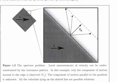
There are a number of problems to be overcome in order to compute the optical flow from the changes in the luminance distribution. Firstly, we can only recognise and compute the motion of patterns in the luminance distribution, not isolated points. This means th a t the luminance information must be combined in some way over a finite spatial neighborhood around each point at which we want to measure motion. The so-called aperture problem arises when we try and measure the two components of image velocity
using a neighborhood that does not contain sufficient luminance structure
[Wallach76][Horn81][Adelson82]. In such situations, we are unable to constrain the measurement to a single solution (figure 1.2). Increasing the size of the neighborhood can permit us to constrain the measurement, but pooling information over a large region increases the likelihood of pooling over motion boundaries and over-smoothing the results, this has been referred to as the general aperture problem [Ong99].
F ig u re 1.2 T h e a p e rtu re problem . Local m e asu rem en ts of velocity can be u n d er co n stra in e d by th e lum inance p a tte rn . In th is exam ple, only th e co m p o n en t of m otion n o rm al to th e edge is observed (V„). T h e co m p o n en t of m otion parallel to th e g ra d ie n t is unknow n. All th e velocities lying on th e d o tte d line are possible solutions.
process. Firstly, the estimation of the velocity field using optical flow is an ill-posed problem since there are an infinite number of velocity fields th a t can cause the observed changes in the luminance distribution. Secondly, there are an infinite number of 3- dimensional motions in the real world th a t could yield a particular velocity field. External knowledge about the behavior of objects in the real world, such as rigid body motion constraints, are required in order to make use of optical flow. Despite the problems, the optical flow information is a rich array of vectors th a t has both local and global properties [Koenderink86]. The optic flow field can thus be subjected to many higher-level interpretations [Nakayama85][Mitiche96][Campani92], the uses of which include:
• Image Segmentation Motion boundaries between different parts of a visual scene can lead to discontinuities in the optic flow, which can provide cues for image segmentation [Campani92] [Smith95].
• Tracking The pursuit of a moving target requires information on its dynamical behavior [Daniilidis98] [Smith95] [Buxton95].
• Shape from Motion The fact th at image motion provides depth cues was observed over a century ago by Helmholtz [Helmholtz62]. Since then numerous experiments th a t highlight the ability of the human visual system to gain depth cues from motion have been carried out [Koenderink86] [Mitiche94] [Gupta95].
• Navigation Motion information can be used in the navigation of autonomous robots [Marino01][Higgins01][Weber97], provide time-to-impact measurements [Scassellati99] and allow obstacle detection [Enkelmann91].
• Video Compression The temporal redundancy in image sequences can be exploited using motion compensation coding schemes [Accame98] [Defaux95].
contain movement, the temporal sampling rate of 25Hz used in most cameras often results in inter-frame displacements of many pixels. As discussed in Chapter 2, this causes difficulties when measuring temporal derivatives in gradient schemes and requires larger search areas for matching algorithms.
In practice, for both biological and computer vision systems, the computation of image motion is complicated by the use both spatially and temporally sampled images, the limited dynamic range of sensors and processing elements, the precision of measurements and computations, environmental difficulties such as shadows and reflections and the various sources of internal and external noise.
1.2 T he Neurom orphic Approach
Nature has evolved many solutions for vision processing, each of which is superbly adapted to the needs of the specific organism involved. Insects perform visual homing, interception, navigation, obstacle avoidance and recognition in a way highly sought-after for our robotic systems and furthermore, frequently perform robustly using less than a million neurons [IndiveriOOb]. They must have evolved dedicated visual algorithms or “software” and neuronal architectures “hardware” th a t are highly efficient in terms of
speed, space, energy usage and robustness. These properties are desirable in an
autom ated robot and have driven researchers to try and emulate the robustness and
efficiency of n atu re’s solutions in both software and hardware [HigginsOl]
[Liu00][Indiveri99][Harrison98][Franceschini92]. Recently, the hardware architectures have become increasingly im portant. This is because transistors are becoming smaller and noisier and their inter-connections are becoming far more complicated. There is an increasing problem with synchronising entire chips and current energy efficiency is many orders of magnitude worse than the brain* [Mead90]. The difficulties th a t the visual cortex and brain have already overcome are now emerging as future design problems for computer chip manufacturers.
N ature has provided us with a source of algorithmic solutions and novel hardware architectures to draw upon and copy. It is hoped th a t these “neuromorphic” systems [Mead90] make good primitives for the construction of more complicated systems. For example, autonomous robots can navigate highly successfully using neuromorphic systems based on models of insect vision [Collett02][Weber97][Franceschini92].
As technology becomes more advanced, it is reasonable to tu rn our attention to more sophisticated and versatile biological systems than those of insects in order to try
and solve more demanding visual tasks. Fortunately, there are many interesting
biological vision systems th a t we can draw inspiration from, particularly the one we are most familiar with, th a t of a human. It is difficult not to be impressed by the capabilities of the hum an visual system, its robustness and its versatility. Many of us take for granted the reliable performance of our visual system in everyday visual tasks, which under analysis prove to be of staggering complexity. Although we do not have direct access to the methods used by the brain in recovering image motion, a number of tools have been brought to bear in revealing its secrets:
• Physics - Explains to us the nature of light, optics, and image formation. It provides a model of the real world in which vision operates. We can use physics to constrain our interpretations of an image to those th a t are possible.
• Anatomy - N ature has evolved the physical structures required for vision th a t have provided us with design templates for optics, sensors and com putational architectures [Marr82] [Bolduc97].
• Physiology - The functional behavior of the com putational structures in biological
visual systems can be investigated and copied [Young01][Young93]
[ReichardtGl] [Hubel65].
• Visual Psychophysics - Allows us to probe the performance of a complete visual system by presenting a stimulus and measuring the response or perception.
• Computational Models - Allow us to test our theories regarding the architecture of biological visual systems from which we can compare performances and make predictions.
• Neuropsychology - Investigations of what happens to the brain after injury can be
very revealing. For example, people can become specifically motion-blind
suggesting a specialised neuronal system [Zihl83].
• Brain Imaging - Techniques such as P E T and fMRI allow us to directly measure
The algorithm discussed in this thesis - the Multi channel Gradient Model - has been developed as p art of a research effort aimed at improving our understanding of the hum an visual system. The model also allows us to make predictions th a t can be tested through psychophysical experimentation; for example, the Multi-channel Gradient Model (McGM) predicts three separate motion illusions th a t are observed by humans in experiments [Johnston94]. The goal of the work described in this thesis is to engineer a real-time version of the McGM th a t can be used in real world applications.
It is useful to compare the two vision systems of human and machine using the language of computer vision. The front-end hum an visual system starts with a stereo pair of 10 megapixel variable resolution colour sensors coupled to a real-time auto-iris and variable focus lens, achieving diffraction-limited imaging. The sensor achieves arc-minute resolution in a central region with lower resolution at the periphery thus permitting high- resolution inspection in the direction of gaze whilst maintaining a large field of view
without excessively high bandwidth. The non-ordered distribution of pixels also
eliminates spatial aliasing problems, whilst the continuous capture sensor eliminates temporal aliasing. The real-time auto-iris and auto-gain control permits a working intensity range of some eight orders of magnitude (although the auto-gain is somewhat slow and can take several minutes to fully adjust). Auto-focus ranges from 3cm to infinity. There exist image pre-processing hardware on the sensor array capable of edge enhancement and d ata compression in real-time and the detector system is steerable through two axes at rates of up to 900degrees/sec. The main processor can process every pixel in parallel and employs in a course-to-fme strategy for grouping visual information. Image processing routines involve high order spatio-temporal filtering with filters tuned
to orientation, velocity, size and other local image structures. Full 3-D scene
reconstruction is standard, as are advanced segmentation and pattern recognition routines. The system works in real-time with a varying but small latency no longer th an 100ms.
The typical machine vision system starts w ith a monochrome GGD camera of
about 1 Megapixel resolution arranged in a regular Cartesian grid. Luminance
dominating the least significant bit. Focus and iris settings are often manual and working intensity range is small. Image processing functionality is rarely on-chip except for experimental systems th a t implement very basic functionality at low resolution. Image processing hardware is capable of performing a single vision task such as filtering or segmentation typically in a serial processing architecture.
It is perhaps unsurprising th a t the m ajority of machine vision systems are not robust or versatile enough to operate in real-world situations when we consider the poverty of computer vision systems compared to the human visual system.
There are several directions for neuromorphic vision engineering to improve upon traditional vision algorithms and architectures [Mead90]. Smart sensors or “silicon retinas” implement specialised processing on the sensor itself [Bolduc97] [Arias96]. Alternatively, vision chips implement models of early biological vision in specialized hardware at a later stage [Collett02][Indiveri00][Liu00][Harrison98].
Neuromorphic sensors functionally correspond to imagers coupled to dedicated hardware im plementations of simple machine vision algorithms. The sensors process the luminance values directly, using analogue electronic circuits coupled to the image sensor itself. Since they are analogue and massively parallel, they work in real-time to tu rn images directly into voltage or current signal outputs th a t could be used as useful inputs
into more complicated systems. Sensors have been described which are involved in
measuring motion or motion derived properties. Neuromorphic sensors have been
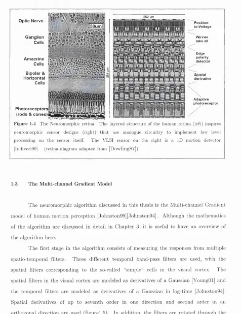
the fly’s elementary motion detector directly into a CMOS sensor using a VLSI process. The parallel architecture of the sensor allows it to operate in real time and provide qualitative motion signals th a t could be used as input to a higher level of processing. A ID neuromorphic sensor system th a t uses adaptive photoreceptors, spatial derivatives and motion detection is capable of tracking high-contrast stimuli has also been described [Indiveri99]. This silicon sensor is based on the structure of a biological retina (figure 1.4) and although the computations are very different to those in biology, it performs focal plane processing in a layered structure in order to build a real-time motion detector into the sensor itself.
Optic Nerve Ganglion Cells Amacrine Cells Bipolar & Horizontal Cells Photoreceptors (rods & cones)
50um? 252 urn
tm
Position-to-Voltage Winner take allEdge polarity detector Spatial derivative Adaptive photoreceptor
Figure 1.4 T h e N eu ro m o rp h ic retin a. T h e layered s tr u c tu re of th e h u m a n re tin a (left) inspires n eu ro m o rp h ic sensor designs (rig h t) th a t use analogue c irc u itry to im p lem en t low level processing on th e sensor itself. T h e V LSI sensor on th e rig h t is a ID m otion d ete c to r [IndiveriOO]. (re tin a d ia g ra m a d a p te d from [D o w lin g S ? ])
1.3 The Multi-channel Gradient Model
The neuromorphic algorithm discussed in this thesis is the Multi-channel Gradient model of human motion perception [Johnston99][Johnston94]. Although the mathematics of the algorithm are discussed in detail in Chapter 3, it is useful to have an overview of the algorithm here.
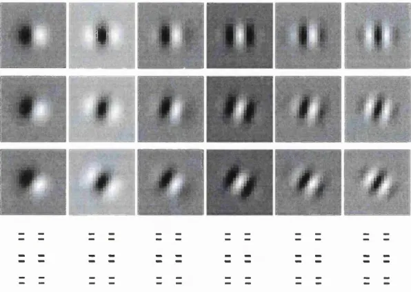
complete range of 360 degrees at 15 degree intervals, simulating the orientation columns found in VI (figurel.6). The strategy of making multiple measurements improves the robustness of the algorithm.
The responses to filters can be used in pairs to compute velocity, although combining the filter responses in a less trivial manner enables a more robust measurement to be made. Several later stages in the model are used to make robust velocity measurements that are immune to static noise. Direction is extracted by observing how the magnitude of velocity varies with the filter orientation, a mechanism that allows the translational component of motion to be separated from the rotational and divergence components [Koenderink86].
Prior to this research, the model had been developed with little thought to optimisation and efficiency. The complete version of the model was time consuming to operate and use, with typical execution times measured in minutes.
•
1
1
: 1.».,.
1
' #
■
*
«
•
1
X*
MM
#
■
1
• 1
Ci
^
1
m
*
4■
'm
m
, e
,«
$
4*
■f*
%
*
F ig u re 1.6 T h e sp a tia l d eriv a tiv e filters are ro ta te d th ro u g h 360degrees in step s of ISdegrees in o rd er to m odel th e o rie n ta tio n colum n found in th e visual cortex. O nly th e first th re e o rie n ta tio n s are show n. T h e to ta l n u m b er of filters em ployed n u m b e rs in th e hun d red s.
1.4 R eal Time Im plem entation
as much as possible. The implementation of a model as complicated as the McGM in real time is a goal th a t is barely achievable using current technology. Using the overview of the algorithm the problems in implementation are seen to be:
• Real-time image acquisition
• Temporal filtering using three derivatives of the Gaussian of log tim e as temporal filters
• Spatial filtering using derivative-of-Gaussian filters at multiple orientations • Large numbers of image arithm etic operations
• Extracting multiple velocity measures
The main com putational bottlenecks are in the spatial filtering operations. The full model uses many (up to 50+) large two-dimensional spatial filters implemented via convolutions, taken at multiple (24) orientations using floating point arithmetic. The higher levels of processing to remove the effects of static noise and non-translational motion components involve a great many arithm etic operations such as m atrix determ inants. Commercial image processing hardware is most efficient at fixed-point integer arithm etic, therefore the effects of reducing the algorithm to use 8-bit or 16-bit precision during both the temporal and spatial convolution stages, as well as the later stages of the algorithm, are examined.
towards migrating the algorithm from the realms of psychophysical model to real-time implem entation and application.
1.5 Thesis Overview
This C hapter has introduced optical flow e l s an estimation of visual motion, its
Chapter 2
Computation of Optical Flow
r » wu«mu%*w(
In this chapter we will examine some of the optical flow algorithms described in the computer vision literature, their biological plausibility and their com putational efficiency. Many diverse algorithms for computing optical flow have been proposed. The designs and solutions draw from many fields of research with artificial intelligence, psychology, image processing, robotics and biological modeling probably the most prolific sources of algorithms. Each field brings its own particular constraints and motivations to the problem, resulting in a plethora of diverse algorithms, but despite this diversity most algorithms for computing optical flow can be placed into one of three categories:
• Pattern Matching Methods. These operate by comparing the positions of image structure between adjacent frames and inferring velocity from change in location. These are probably the most intuitive methods.
• Differential or “Gradient” Techniques work using derivatives of image intensity in space and time. Combinations and ratios of these derivatives yield explicit measures of velocity.
• Motion Energy Methods use space-time oriented filters tuned to respond optimally to specific image velocities. Banks of such filters are used to respond to a range of possible visual motions.
suitable to small inter-frame displacements, where ‘small’ and ‘large’ are relative to the size of the local filters being used [Yacoob99]. In a biological sensor there is no uniform, clocked temporal exposure or “frame rate” as there is in a camera. Instead, the sensor (retina) is exposed continuously over time, allowing it to sample temporal information much more effectively. This suggests gradient or energy methods are suitable for motion estim ation in biological systems. In machine vision applications we use CCD cameras w ith a discreet sample rate, implying th a t varying image velocities will result in varying inter-frame displacements - if these displacements are too high then a gradient method will fail as the smooth continuity of the space-time image breaks down. Although we can use strong spatial anti-aliasing (blurring) to remove temporal aliasing [Christmas98] it has the side-effect of degrading spatial information. Thus for a given spatial resolution, we are forced to sample at a minimum frame rate. This implies th a t in a real-time system we must also compute optical flow at the same minimum frame rate. In effect, measuring optical flow with a gradient technique becomes more robust the faster the frame rate at which we can compute the gradients (up to a limit where the temporal differences are immeasurably small [Yacoob99]).
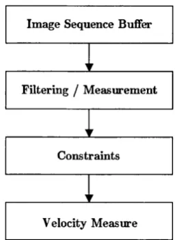
Many algorithms follow a similar functional architecture (figure 2.1). Firstly, the image sequence or temporal buffer is somehow filtered to extract basic measurements. This may be through filter convolutions, Fourier transforms, pattern extraction, arithm etic operation etc. The measurements are then recombined using a diverse range of
methods to achieve a basic (usually flawed) velocity measurement. The final flow
estim ation is made possible by enforcing a set of constraints on the measurements and results. The constraints are generated through hypotheses on the nature of the flow or motion (such as rigid body motion constraints), but even w ith constraints the information recovered is not usually complete enough to compute a unique solution to the optic flow field. It was shown in Chapter 1 th a t optic flow is the motion estimated from the observable changes in the luminance p attern over time and th a t an example of an
zero. Another complication is th a t there exists no unique image motion to explain an observed image brightness change. Thus the measurement of visual motion is frequently impossible and always has an infinite number of physical interpretations.
Image Sequence Bufifer
Velocity Measure Constraints Filtering / Measurement
Figure 2.1 Basic functional architecture for computation of optical flow found in many algorithms
2.1 Elem entary Visual M otion Models
Despite the difficulties in the recovery of optical flow, biological vision systems are remarkably good at recovering visual motion. This is because, in the same manner th a t biological systems have specialised mechanisms to perceive colour and stereopsis, they have also evolved dedicated mechanisms to detect visual motion [Albright93]. As in other areas of com putational vision, it is beneficial to build models of these natural systems to
provide inspiration in overcoming the problems. From psychophysical and
obstacle for the engineers however, is th a t the com putational models of biological vision systems are often very complicated and have not been optimised for speed.
One of the earliest biologically plausible visual motion sensors was proposed by Reichardt [Reichardtbl]. The detector consists of a pair of receptive fields, the signal from one of which is delayed with respect to the other before combining in a non-linear
AS
AT
AT
Figure 2.2 The Reichardt elementary motion detector. Receptors 1 and 2 (shown as edge detectors) are separated in space by a distance AS. A delay is imposed on each signal and the result combined at location C through a multiplication. Finally, the result from one half of the detector is subtracted from the other to increase directional selectivity.
(e.g. multiplicative) way. The two halves are then subtracted at the summing junction to increase directional selectivity. The sensors in shown in figure 2.2 are Laplacian edge detectors although they could be any spatial filter or feature detector. One of the drawbacks of the detector is th a t a strong signal can results from a high contrast input, even if the correlation is not particularly good. Additionally, the detector is not able to recover velocity directly. Banks of detectors tuned to many speeds and orientations are required, the interpretation of which can be ambiguous.
sophisticated models of biological vision [Beare99] [Zanker96] and current VLSI technology is now able to implement low resolution detectors on the CCD sensor dye itself [Arias96].
2.2 Change D etection
Consider the relatively simple case of segmenting moving regions from static regions in an image sequence. A binary image indicating moving/non-moving regions is sought, from which further analysis (e.g. blob analysis) can be made (figure 2.3). The process would seem intuitively easy - we are simply looking for changes in image intensity above some threshold th a t we presume to be caused by a moving object in the visual field. However, the number of false alarms th a t arise from sources such as sensor noise, camera motion, shadows, environmental effects (e.g rain or reflections) and illumination changes cause great difficult in robust motion detection. Again, there is opportunity to learn from biological systems, which, despite being very sensitive to motion are very robust to noise and “uninteresting” visual events.
This technique is now employed in surveillance situations in which detection of movement is an interesting event th a t should be brought to the attention of an operator for further investigation. However, due to the problems dealing with a complicated real- world environment, the robust detection of genuine movement a difficult task th a t has attracted attention from researchers [Rosin98] [Stuart99].
Figure 2.3 L e/f;C om posite of 5 fram es from an im age sequence of a person w alking
across a car park. Hz^/i^/Difference im age betw een first an d second fram e. [Rosin98]
2.3 Correlation Methods
Correlation or “P attern Matching” methods are perhaps the most intuitive method for computing optical flow and recovering speed and direction of movement. They work by selecting features in one frame of an image sequence and then searching for these features in a subsequent frame (figure 2.4). Changes in position indicate movement over time, which is velocity. The problem of matching features in temporally separated frames is similar (although less constrained) to the spatially based “correspondence” problem encountered in stereo vision - feature pairs are difficult to find and match robustly and accurately.
These algorithms are usually characterized by slow execution times due to their iterative and exhaustive searches. A brute force search algorithm th a t attem pts to match via correlation requires a prohibitive amount of computation. If the image size is M * M the search templates are N * N , and the search window is L * L then the total
com putation required would be For a 512x512 image, 10x10 pixel block
attem pt is usually made to narrow down the search domain [OhOO] [Anandan93] [Accame98] but it stills remains a computationally expensive design.
Template
S earch Window
—i *
F ig u re 2.4 M otion estim a tio n v ia in te r fram e co rrespondence, (left) A te m p la te is selected in an early fram e. In a su b se q u en t fram e th e te m p la te is m a tch e d to th e tra n s la te d fea tu re in th e new image.
One of the most common uses of block-based correlation motion computation is for real-time video encoding [Accame98][Defaux95]. The enormous growth of multimedia and digital video coding in recent years has increased the amount of effort being directed into
video compression technologies. One of the key redundancies exploited in video
compression is the similarity between temporally adjacent images in a sequence. Less bandwidth is required to transm it the differences between subsequent images than the entire images themselves, even less image data is necessary if the motion and deformations needed to warp from one frame to the next is known. The algorithms that enable this motion-compensated compression are usually based upon block-based matching due to their computational simplicity. Consequently, many optimisations and implementations have been developed in order to reduce the search space [OhOO] and increase the speed of these algorithms [Accame98j.
2.4 Spatio-tem poral Methods
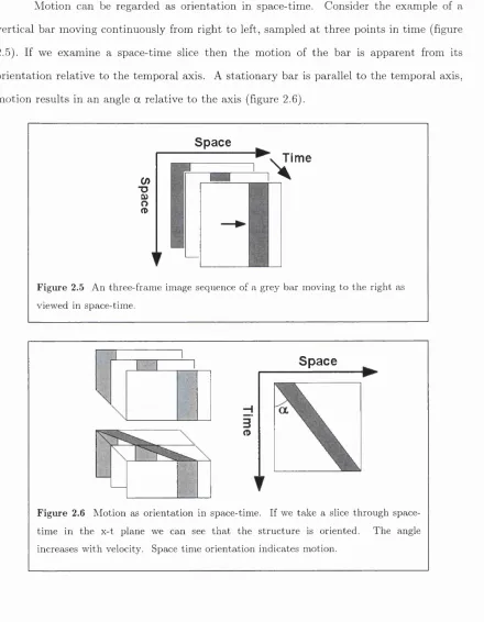
Motion can be regarded as orientation in space-time. Consider the example of a vertical bar moving continuously from right to left, sampled at three points in time (figure 2.5). If we examine a space-time slice then the motion of the bar is apparent from its orientation relative to the temporal axis. A stationary bar is parallel to the temporal axis, motion results in an angle a relative to the axis (figure 2.6).
Space
(/) ■o % (D
V Time
X
Figure 2.5 A n th ree -fram e im age sequence of a grey b a r m oving to th e rig h t as view ed in space-tim e.
S p a c e
o
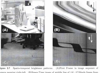
Figure 2.7 shows the space-time brightness changes of the central horizontal line of pixels from two image sequences. In the left image is a single frame from the sequence, in the right image, the horizontal axis is the central line from each frame and the vertical axis becomes time. In the case of a simple camera pan shown in figure 2.7(A) it is possible to interpret the space-time diagram (figure2.7(B)) by observing the slope of the lines. This structure is indicative of velocity and designing a motion detector based on the measurment of spatio-temporal orientation is an apparent possibility. However, when observing the entire three-dimensional space-time cube of an image sequence consisting of multiple motions, occlusions, uncoverings, illumination changes, shadows and noise, the sheer complexity of the spatio-temporal brightness pattern is an indication of the difficulty in recovering optical flow.
s i
F ig u re 2.7 S p a tio -te m p o ral b rig h tn e ss p a tte rn s . (A )F irs t F ra m e in im age sequence of c a m e ra p an n in g rig h t-left. (B )S p ace-T im e im age of m iddle line of (A). (C )Single fram e from sequence w ith p erson w alking left to rig h t. (D )S pace tim e im age of m iddle line of (C).
model (figure 2.8). In the gradient model the ratio of a spatial and temporal filter pair is used as a velocity measure. In the motion energy model many filters of tuned spatio- temporal orientation are employed in order to determine the velocity. Both schemes use
filters of a type that is known to be abundant in the human visual
system[AdelsonS5][Young93]. Although there is debate over which scheme is used in the human visual system, it is possible to synthesize the oriented filters in the motion energy model from space-time separable filters [Fleet89][Huang95]. It is also interesting to note th at spatial filters of similar types have been shown to dominate the components of image structure found by performing an independent component analysis [Hateren98].
Space
H 3 (D
Ratio
Space
►
H 3 o
Orientation
F ig u re 2.8 Low level sp a tio -te m p o ra l filter models. T h e ellipses re p re se n t th e positive an d negative lobes on a sp a tio -te m p o ra l filter. T h e filters on th e left w ould form p a r t of a g ra d ie n t m eth o d , th o se on th e rig h t w ould be from a m otion energ)' m ethod.
We will first examine the gradient model, the formulation of which relies on the assumption of intensity conservation over time [Horn81]. The assumption is th a t over short periods of time changes in intensity are only due to translation and not changes in illumination, reflectance etc. The assumption asserts th at the total derivative of image intensity of time is zero at every point in space-time. Thus if the image is parameterised as
d l ( x , y , t )
Differentiating by parts leads us to the Motion Constraint Equation, the fundamental tenet of the gradient method:
d l dx d l dy d l dt
dx dt dy dt dt dt (2.2)
6 / a / a / ^
U H V + = 0
dx dy dt (2.3)
Where w = and v = . The parameters ( x , y ,t ) have been omitted for clarity of
notation. Since there is only one equation with two unknown velocity components, we can only recover the component of velocity v,, , which is in the direction of the luminance gradient:
-SO
% )
(2.4)
There are a number of problems with the Motion Constraint Equation. Firstly, it is a single equation with two unknowns {u and v) and is thus under-constrained and insufficient to compute optical flow. Using (2.3) alone will only yield a linear combination of the velocity components - it is a m athem atical statem ent of the aperture effect mentioned in chapter 1. W ith the basic motion constraint equation the aperture effect is caused by the single measurement, rather than being a product of degenerate image structure.
A second problem becomes apparent if both the spatial gradients or I y become small or zero, in which case the equation becomes ill conditioned and computed velocity approaches infinity. These regions can be seen in figure 2.9 (C) and (D) where some areas have become a uniform mid-grey which corresponds to no gradient information. Additionally, the intensity derivatives themselves are problematic to perform in a stable manner. The im plem entation of the partial derivatives is achieved through convolution with differentiating filter functions, such as the Sobel, Prew itt or Differential of Gaussian. Since we are utilising numerical derivatives of a non-continuous (sampled) “image function” , the accuracy of the derivatives is better for smaller spatio-temporal intervals. If we undersample space-time, the problem of aliasing in the image, especially in temporal domain when frame rates are usually low, needs to be taken into consideration. For fast image motions the sequence is usually highly temporally undersampled making the tem poral gradient measurement poor. Ideally, the sample rate should be high enough to reduce all motions to less than one pixel per frame, so th a t the numerical temporal derivative is well conditioned.
The spatio-temporal derivative filters required to implement gradient algorithms resemble those found in the visual cortex, although the best functional form is still
controversial [YoungOl]. An advantage of the gradient scheme over motion-energy
An anomaly in the gradient scheme is its ability to extract velocity of a moving linear luminance ramp - something th a t is poorly sensed by biological systems [Nakayama85]. A translating linear luminance ramp produces the same stimulus as a luminance ram p undergoing a global change in brightness. It is interesting th a t a biological system would benefit from being insensitive to such changes since global illumination changes occur regularly with natural lighting. A solution to this problem might be achieved through appropriate pre-filtering. Since the local spatio-temporal structure of a luminance ram p is the same at all locations, it would elicit a uniform response from temporal and spatial band-pass filters. If such filters were to be used as a preprocessing stage, their output image would be w ithout structure, rendering the motion of the ram p invisible to a subsequent motion detector.
2.5 Im proving th e M otion Constraint Equation
It has been shown in the previous sections th a t the basic Motion Constraint Equation (MCE) has several shortcomings th a t need to be overcome in order to compute optical flow. Many methods have been adopted in order to improve upon the basic MCE, most of which apply additional constraints in order to solve for the two velocity components u and
V.The methods involve measuring more information to gain extra images, extracting
more information from a single image, or applying physical constraints in order to generate additional M C E's.
gradient equation can be solved analytically. W ith additional functions an over constrained set of equations can be constructed:
dx dy dt
dL dL d l
u-\— -v + - 2 _
dx dy dt
0
(2.5)^ M + ^ V + ^ = 0
dx dy dt
which can be re-written as a m atrix to be solved via a mechanism such as linear least squares [Simoncelli91] or total least squares [WeberQl]
where:
A»v = b
A =
v = A - ' b
<
dx dy dt
5 . 5 . d l.
dx dy b = — dt
K E u
dx dy_ _ dt _
(2.6)
(2.7)
This method relies on the M atrix A being invertible (non-singular), which it will not be in m any regions of the image if there is a lack of image structure, such as a purely 1- dimensional grating.
• Performing global optimisations (e.g, smoothness) [Horn81][Nagel83][Heitz93] • Constraining the flow to a specific (e.g affine) model [Liu97] [Ong99] [FleetOO] • Using multiple spatial and temporal scales [Anandan89][Weber94][Yacoob99] • Exploiting temporal consistency [Giaccone97] [Giaccone98]
The MCE of equation (2.7) can also be solved by making more measurements or obtaining more information from the image by:
• Applying multiple filters [Mitiche87][Sobey91][Arnspang93][Ghosal97] • Using neighbourhood integration [Lucas81][Uras88][Simoncelli91] • Using multi-spectral images [Golland97]
Global Optimisation
The estimation of a dense velocity field is usually made difficult due to the lack of inform ation and spatial structure in an image. In order to “fill-in” the gaps in the velocity field several global constraints have been applied, the general idea of the global optim isation is th a t the original optical flow field, once computed, is then iteratively regularised with respect to some smoothness constraint.
The first global constraint was proposed by Horn and Schunk [Horn81], with the velocity smoothness term being given as:
^Sm oothness I I dx )
du
+ — +
y d x ) y d y y (2.8)
The error £ in the MCE was then minimized with the addition of this smoothness constraint:
2
where X dictates the relative importance of the smoothness term , is the spatial derivative in the x-direction, in the y-direction and is the temporal derivative. The
algorithm is able to fill in regions with small gradients and produces smooth, noise free results, however, the degree of blurring over motion discontinuities is a major drawback. In order to overcome this problem Nagel [Nagel83] introduced second order derivatives and an oriented smoothness constraint th a t attenuated the smoothing term in the direction for which the gradient was well conditioned [Nagel83]. This mechanism meant th a t smoothness was not imposed across steep intensity gradients (edges) in an attem pt to handle occlusions, and th a t smoothness was applied where it was needed, i.e in the direction tangential to the gradient.
The psychophysical theory of edge detection in static images has been developed extensively and the extension of edge theories to the time domain can be used in the
measurement of optic flow. The method of Hildreth [Hildreth84] is based on the
Laplacian of the Gaussian, previously used in determining the location of edges and contours of significant intensity change. Hildreth computes motion vectors on the edges produced from the Laplacian filtering operation and then minimizes the variation in velocity along the contours to solve for the aperture effect.
The optical flow resulting from global constraints are often more robust due to the pooling of results, as well as being more pleasing to the eye. Two major drawbacks are th a t their iterative nature often requires prohibitive amounts of com putation time, and motion discontinuities are not handled correctly so th a t erroneous results are produced in the regions around motion boundaries. In order to alleviate the problems other techniques have been proposed using global statistics such as Markov Random Fields [Heitz93], which are able to preserve motion boundaries.
Neighourhood Integration
motion is consists of a pure translation within the local region. The constraints are usually weighted using a m atrix W ( x ,y ) such as to bias the results from nearer the center of the local region, for example, the weight m atrix can be a Gaussian. The MCE is then w ritten a minimization problem:
x,y eC l
where error term £ is then minimized, or the set of equations solved through a variety of numerical techniques.
Motion Models
The neighourhood integration techniques, when attem pting to solve the MCE, assume th a t the image motion in local regions is purely translational. More advanced motion models (such as the affine model) are able to cope with a greater range of image motions as well as provide additional constraints.
The method usually involves restating the MCE with an error function £ th a t can be solved or minimized in a least squares manner [Campani92] [Bergen92] [Cupta97] [Ciaccone97] :
+ V + (211)
x,ye Cl
Here the MCE is not assumed to be zero but is a function to be minimized over some local region Q . This local region can have more th an just translational components to its flow. The velocity components are thus modeled using param eters from a local or global motion model of varying complexity, from the 2-parameter uniform translation to the 6 param eter
affine transform. A simple motion model taking into account rotation, scaling and
(2.12)
The error in the MCE in equation 2.14 is then minimized by solving for the param eters a, b and c. These param eters express the local flow in term s of translation, rotation and divergent motion.
Giaccone [Giaccone97] develop an algorithm m otivated by segmenting foreground and background (e.g. actors from scenes) and the segmentation of regions in image
sequences, using a rigid motion model to constrain the system of equations. The
displacement in a small region is modeled by an eight param eter transform of the form:
u
=
+
a^xy
+
a^x + a^y + a^)
V =
{a^xy
+a^y^
+a^x + a^y + a^)
(2.13)
which is derived from a global motion model, with the assumption th a t the changes in world coordinates position between frames are small.
G upta and Kanal [Gupta97] start by integrating the MCE over a space-time volume V :
[ ( < + v / , + / , ) d F = 0
(2.14)They then utilize Gauss’s divergence theorem to reduce this expression to a surface integral. The MCE then becomes:
uidydt
+
vidxdt
-
I{u^ + )dxdydt
+
Idxdt
= 0
(2.15)This is followed by a constraint th a t the flow is linear in a small space-time neighborhood:
u{x,
y , t ) = UyX -\- a ^ y + a^t +v(%, T» 0 = ^1^ + h^y -V b-ft +
the problem is then reduced to determining the flow coefficients and . They substitute these equations for u and v into their integrated MCE and solve using a least squares method. The robustness of this algorithm lies in the integration stage th a t obviates the need for taking spatial dérivâtes thus avoiding the associated problems. However, despite the lack of filtering, the integrals are still time consuming to compute - the execution time is stated as approx 1 m inute for a 512x512 image on a Sparc station.
The 2D affine flow model can be expanded upon further by employing a complete motion model to parameterise any arbitrary 3-D steady motion under perspective projection, thus recovering optical flow as well as other useful real world motion param eters [Liu97].
Multiscale Methods
Large inter-frame displacements cause standard gradient methods to behave poorly. This is because the image sequences are usually temporally under-sampled causing the temporal derivative measurements to break down, the only solution to which is to use very large spatial filters [Christmas98]. The utilization of a Gaussian pyramid architecture has the benefit of coping with larger inter-frame motions and filling in the gaps left in large regions of uniform texture. If the gradient method is to be used when large spatial motions are present then a course-to-fine pyramid estimation scheme is usually employed [Zhang01][Mahzoun99]. In this scheme, coarse scale motion estimations are used to seed progressively finer scale measurements.
A temporal multiscale approach [Yacoob 99] also allows for a large range of image motions to be computed accurately, although this method requires using a frame rate high enough to reduce the fastest motions to approx 1 pixel/frame.
Temporal Consistancy
forward architecture which is able to address the im portant issues of multiple motions, large scale motion and segmentation of consistently moving regions. They use a least squares solution to an affine model, with the error function given by;
s = Y , e ( x , u , ( x ) f
(2.17) e(x,u , ( % ) ) = / , ( T ) - /,_!(x - M , ( % ) )
W here x = ( %, y ) and the term (x — m, (%)) is the previous image at time ^ — 1
projected forward to the current image at time t using the velocity information w,(x) . The algorithm is shown to be highly robust to a range of velocities and performs well compared to simple affine models. The com putational overhead is somewhat burdened by the generation of the projected image, for PAL sized images a com putation time of 34 seconds per frame is quoted.
Multiple Filters
A single MCE is not in itself sufficient to compute optical flow. The under constrained MCE can be easily improved upon by noticing th a t its differentials ^ (where
X; = — y ) provide additional solutions to the optic flow vectors v :
( - )
This method was first used by Nagel [Nagel83] using second order derivatives. In fact, the differentiating operator is just one of an infinite number of operators which can be applied in order to generate multiple M CE’s. Usually the operators are applied numerically via convolution with a suitable filter, and since convolution is a linear operator we can write:
_ ^ . d l , dl , dl ]
(90, ^
= 0
V
4-dt
(2.19)
7 1 = 0
where O, is an arbitrary convolution filter (e.g. Gaussian, Differential of Gaussian, averaging, Laplacian etc) and 0 denotes the convolution operator. This process works because convolution does not change the orientation of the space-time structure. It is im portant to employ filters th a t are linearly independent otherwise the additional M CE’s produced will be degenerate and nothing will have been gained. The filters and their differentials can be pre-computed for efficiency, and a massively parallel im plementation is possible since the operators are local.
Again, using two such filters to generate two equations then gives enough information to solve for the velocity components analytically (provided the measurements are not degenerate), unless the image itself is degenerate as in the case of a ID grating.
make two MCE equations th a t they then solve analytically. However, a problem with using just two M CE’s is th a t the derived analytical solution is of quotient form for which the denominator can become zero in regions of low spatial structure. Although they also estim ate the condition number of the m atrix to test if the solution is well conditioned, it does not solve the problem.
Usually, more th an two such equations are generated providing an over constrained system of linear equations [Nagel83][Weber94]. Weber et al [Weber94] convolve the input image sequence with a set of Gaussian derivatives of first and second order at a number of orientations and scales to provide a system of linear equations. Each pre-filtered image /. is differentiated with respect to x, y and t to provide the set of M CE’s. They then use a total least squares method to determine the velocity components, rejecting the results from filter scales for which the model has failed. This model uses a similar filtering stage to the McGM and similar processing demands are required. The com putation time was stated at 4 minutes per frame on a Sparc 1 workstation, although a massively parallel implementation using a CM5 Thinking Machine with 128 processors was able to cut this to lOseconds per frame.
Most of the existing optical flow techniques depend on the conservation of
intensity or intensity-derived values. Ghosal and M ehrotra [Ghosal97] present an
algorithm based on the orthogonal Zernike moments (usually used to describe optical
aberrations) of image intensity. Zernike moments are rotation and virtually scale
invariant, resulting in features which are well conserved during motion. Additionally, since the moments are integral based they are robust to uncorrelated noise. The M C E 's generated are thus based on the moments M 'o f the image:
= 0 (2.20)
dx dy dt
the velocity components. The algorithm is relatively slow due to the integration required in extracting the Zernike moments and the overhead of the SVD routine - 71 seconds were quoted as required for a 233x256 image.
The approach of using multiple filters is certainly biologically plausible. Biological vision systems are known to be massively parallel and are highly suited to filtering operations, with many of the filters used being of the type found in the human visual system. The multiple projections from the LGN and the layers of cells in the visual cortex are known to act as local filters. Applying these filters is simply a m atter of replication, an efficient architecture to implement in the connection rich visual cortex. How these responses are re-combined to give us such a robust motion perception is still very much an area of active research. The task of m atrix inversion for solutions of multiple equations is rather less plausible (although not impossible) and other models are usually considered, which we will discuss in the next chapter.
Multispectral Methods
If multi-spectral images are available then they can be used to generate several different brightness functions. For instance, the separate red, green and blue colour planes from a standard colour camera can be treated as three independent images, yielding three motion constraint equations th a t can be solved. A problem with this simple method is th a t the colour planes are usually highly correlated, a fact which is exploited in most colour image compression algorithms. In these situations the linear system of equations can often be degenerate. The improvement in the quality and robustness of optical flow measurement does not w arrant the extra expense in computation.
Using these measures it is possible to improve greatly upon the simple RGB method [Golland97].
2.6 M otion Energy M ethods
We have already seen (section2.4) th a t motion can be regarded as orientation in space-time and th a t the gradient method extracts this orientation through the ratio of spatially and temporally tuned filters. The “motion energy” , or “frequency-based” models are in many ways similar to gradient models in th a t both schemes employ banks of filters to extract this space-time orientation and hence signal motion. The main difference is th a t the filters used in motion energy schemes are designed to respond to specific spatio- temporal orientations rather than using the ratio of spatial and temporal filters.
The design of spatio-temporally oriented filter is usually carried out in frequency space due to the following relationship between a translating 2-D pattern and its Fourier transform:
I { k ,(D) = Iq( k) S( CD + V » k )
where is the Fourier transform of the static pattern, x = ( x , y ) is image position, k = { k ^ , k2) is spatial frequency, t is time, Ct) is temporal frequency and v = (m,v) is
one particular velocity. This process of designing the filters in the Fourier domain has led to these schemes being labelled as “Frequency Based” . Additional complications are th at the filters are phase and polarity dependant and so their output depends on how a pattern lines up with the receptive field at any one time, and the polarity of the stimulus. For example, a moving bar would elicit a response th at oscillates over time, and inverting the polarity of the bars contrast would invert the response. To overcome these problems, the filters required are usually designed as quadrature pairs [Adelson85], the response from which is squared (or passes through some other non-linearity [Simoncelli98]) and summed to produce the so called “motion-energy” measure th a t is phase independent.
S p a c e
H
3
o
Figure 2.10 A space tim e o rien ted filter resp o n d in g to a m oving edge. In th e frequency dom ain, th e m oving edge has its co m p o n en ts c o n stra in e d to a line. T h e sp ace-tim e o rien ted filter has a frequency response ce n te re d on th is line.
A quadrature pair responds maximally to only one pair of points along the line in frequency space. Banks of filters are required because a quadrature pair will be optimally tuned for one velocity whilst still having a (reduced) response to a range of non-optimal ones (figure 2.11). Designing the filters to be more tightly tuned to a narrower range of velocities implies th a t more filters are required to span velocity space, this is the velocity specificity problem. In addition, filters must remain sensitive to a range of spatial orientations and scales, thus many extra filters are usually required and the filtering
requirements quickly become computationally demanding. Another problem is that
contrast is low or the velocity is not near the detectors peak sensitivity. Additional confusion arises between velocity and spatial and temporal frequency. In order to disambiguate velocity from other parameters, some comparison of all the different responses (normalisation) is required [Simoncelli98],
S p a ce S p a ce ^
--- 7— S p a ce ^
H H H 3 fl> 3 o 3 o 0% 50% 100%
F ig u re 2.11 Left: A sp ace-tim e o rien ted filter resp o n d s o p tim ally to a n arro w ran g e of v elo cities/sp ac e-tim e o rie n ta tio n s b u t will still p a rtia lly respond to non- o p tim al velocities (center). In o rd er to d e te rm in e th e velocity som e n o rm a liz a tio n / com parison schem e is usually required