1
Pendulum Base using H
Optimal Loop Shaping Controller with
First and Second Order Desired Loop Shaping Functions
Mustefa Jibril1, Messay Tadese2, Reta Degefa3
1 Msc, School of Electrical & Computer Engineering, Dire Dawa Institute of Technology, Dire Dawa,
Ethiopia
2 Msc, School of Electrical & Computer Engineering, Dire Dawa Institute of Technology, Dire Dawa,
Ethiopia
3 Msc, School of Electrical & Computer Engineering, Dire Dawa Institute of Technology, Dire Dawa,
Ethiopia
Abstract
In this paper, a horizontally moving suspended mass pendulum base is designed and controlled using robust control theory. H optimal loop shaping with first and second order desired loop shaping function controllers are used to improve the performance of the system using Matlab/Simulink Toolbox. Comparison of the H optimal loop shaping with first and second order desired loop shaping function controllers for the proposed system have been done to track the desired angular position of the pendulum using step and sine wave input signals and a promising result has been obtained succesfully.
Keywords: Pendulum, H optimal loop shaping, Track 1. Introduction
A pendulum with suspended mass is a system that has a mass suspended in its base and a mass suspended from a pivot so that it can swing freely. When the suspended mass in the base of the pendulum forced to move horizontally by applying a force, the pendulum become displaced sideways from its resting, equilibrium position, then the pendulum will be subjected to a restoring force due to gravity that will accelerate it back toward the equilibrium position. The restoring force acting on the pendulum's mass causes it to oscillate about the equilibrium position, swinging back and forth. The time for one complete cycle, a left swing and a right swing, is called the period. The period depends on the length of the pendulum and also to a slight degree on the amplitude, the width of the pendulum's swing.
2. Mathematical Modeling of the System
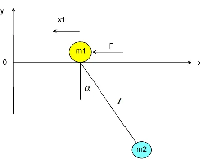
A system consists of two point masses, m 1 and m2, connected with a weightless rigid rod of length
l (Figure 1). The motion occurs in a gravity field and is considered to be in a plane, i.e. is considered in the coordinates x, y, t. The location of point of a mass m1 (suspension) is not fixed, and can move along the axis x. The mathematical model of the system will be as follow.
2
Figure 1 Pendulum with suspended mass
The four functions of time of the system are, x1(t), y1(t), x2(t), y2(t), i.e. the Cartesian coordinates of the first and second points.
The suspension cannot move vertically Y1=0
While the second is described by equation
2 2 21 2 2
x x y l
We choose the generalized coordinates as q t1
x t and q t1
2
t where is the angle between the vertical is and the axis of rod.1 1, 2 1 sin 2, 2 cos 2
x q x q l q y l q
The kinetic energy of system T = T1+ T2 in coordinates q1, q2. For the suspension we have
2
2 2
1 1
1 1 1 1
1 1
2 2 2
x
m v
m v m x
T
For the pendulum we obtain
2
2 2
2 2 2
2 2 2 2
2 2 x y
m v m
T v v
V2x and V2y simply simplified as
2 1
2
cos
sin
x y
v x l
v l
Rewrite T2 as function of and x1
2
2 2
2 1 2
2 2 1cos 3
2 2
m x m
T l x l
For the force of gravity F2 acting on the pendulum. For its projection we have
2 2
2 0
gx
gy
F
F m g m
y
3
In coordinates q q1, 2
y2 is expressed by the formula
2 2 cos
4V q m l g
In so far as the considered motion is potential, it is necessary to use the Lagrangian equations
1 2
L T V T T V Or
2 2
1 2 2
1 2 1 cos 2 cos 5
2 2
m m m l
L x l x m l g
Differentiating L byq q q q1, 1, 2, 2, (recall, thatq1x q1, 2 ) we obtain
1 2 1 2
1 1
2 1 2 1
2 2
0, cos
sin , cos
L L
m m x m l
q q
L L
m l x g m l l x
q q Then 1 1
d L L
F
dx q q
2 2
0
d L L
dx q q
Substituting the obtained expressions into Lagrangian equations and differentiating them by t, we come to two equations with respect to x1 and
2
1 2 1 2 cos 2 sin 6
m m x m l m l F
1cos sin 0 7
x l g
Linearizing the above equation as
2 cos 1 sin 0
After linearization, Equation (6) and Equation (7) becomes
1 2 1 2
1
8
0 9
m m x m l F
x l g
Let
1 1, 2 1, 3 , 4 , 5
4
2
1 2 1 2
0 1 0 0 0 0 1 0 0 0 0
0 0 0 1 0 0 0 0 0 0 1 0 0 0 0 0 0 0 0 0 1 0 0
m l
m m m m
z F
y z
The parameters of the system are shown in Table 1 below. Table 1 Parameters of the system
No Parameter Symbol Value
1 Suspended mass m1 0.4 Kg
2 Pendulum mass m2 0.2 Kg
3 Rod length l 0.4 m
4 Gravitational constant g 10 m/s^2
The state space representation of the system then becomes
0 1 0 0 0 0
0 0 0 0 1.33 1.67
0 0 0 1 0 0
0 0 0 0 1 0
0 0 0 0 0 0
0 0 1 0 0
z F
y z
3. Proposed Controllers Design
3.1H Optimal Loop Shaping Control
H Optimal Loop Shaping Control computes a stabilizing H∞ controller K for plant G to shape the sigma plot of the loop transfer function GK to have desired loop shape Gd with
accuracy γ = GAM in the sense that if ω0 is the 0 db crossover frequency of the sigma plot of Gd(jω), then, roughly,
0
_ _
0
_ _
1
d
d
G j K j G j for all
G j K j G j for all
A MIMO stable min-phase shaping pre-filter W, the shaped plant Gs = GW, the controller for the
shaped plant Ks = WK, as well as the frequency range {ωmin,ωmax} over which the loop shaping is
5 Controller
In this paper, the plant has been desired loop shaped with a first order and second order system. For the first order, the desired loop shaping function is
1
1 1
d
G s
And the H Optimal Loop Shaping Controller becomes
6 5 5 4 4 3 3 2 21
5.369 4.409 9.094 1.764 1.399 3.415
1.639 1.007 2.751 2.820 2.818 6.955
s s s s s
s s s
K
s s
s
s
For the second order, the desired loop shaping function is
2 2
1
2 6
d
G
s s
And the H Optimal Loop Shaping Controller becomes
8 7 7 6 6 5 5 4 3 3 2 22 4
7.314 3.221 2.645 5.459 1.123 2.353 6.077 1.222
1.639 1.007 2.753 2.826 1.153 2.867 3.523 8.939
s s s s s s s
s s s s s s s s
K s
4. Result and Discussion
Here in this section, the investigation of the open loop response and the closed loop response with the proposed controller have been done. Finally the comparison of the system with the proposed controllers for a first order and a second order desired loop shaping design have been done.
4.1Open Loop Response of the Pendulum
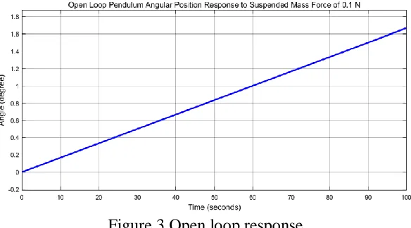
The open loop response of the system for a 0.1 Newton suspended mass force simulation is shown in Figure 3 below.
Figure 3 Open loop response The pendulum angular position angle increases for the 0.1 N input.
4.2Comparison of the Step Response of Pendulum with Suspended Mass using H Optimal Loop Shaping Controller with First and Second Order Desired Loop Shaping Function Controllers
6
Figure 4 Step response
The data of the rise time, percentage overshoot, settling time and peak value is shown in Table 2.
Table 2 Step response data
No Performance Data First Order Second Order
1 Rise time 1.05 sec 1.12 sec
2 Per. overshoot 13.3 % 40 %
3 Settling time 1.38 sec 1.45 sec
4 Peak value 17 Degree 21 Degree
As Table 2 shows that the pendulum with suspended mass using H optimal loop shaping controller with first order desired loop shaping function controller improves the performance of the system by minimizing the rise time, percentage overshoot and settling time.
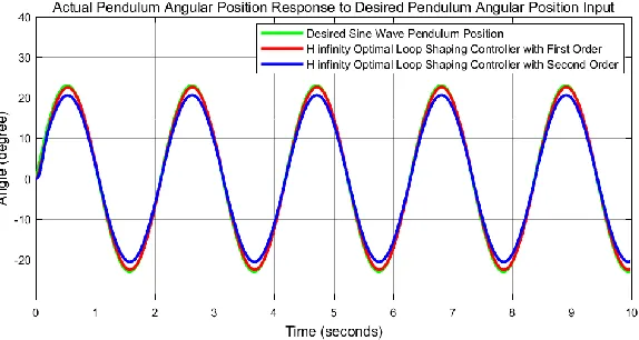
4.3Comparison of the Sine Wave Response of Pendulum with Suspended Mass using H Optimal Loop Shaping Controller with First and Second Order Desired Loop Shaping Function Controllers
The simulation result of the sine wave response of pendulum with suspended mass using H optimal loop shaping controller with first and second order desired loop shaping function is shown in Figure 5 below.
7
controller with first order desired loop shaping function controller improves the performance of tracking the set point input to the system.
5. Conclusion
In this paper, the design and simulation of a horizontally moving suspended mass pendulum base is done using H optimal loop shaping with first and second order desired loop shaping function controllers. Comparison of the proposed system with H optimal loop shaping with first and second order desired loop shaping function controllers have been done to track the desired angular position of the pendulum using step and sine wave input signals. The step input signal response shows that the pendulum with suspended mass using H optimal loop shaping controller with first order desired loop shaping function controller improves the performance of the system by minimizing the rise time, percentage overshoot and settling time while the sine wave input signal response shows that the pendulum with suspended mass using H optimal loop shaping controller with first order desired loop shaping function controller improves the performance of tracking the set point input to the system. Finally the simulation comparison results prove that the system with H optimal loop shaping controller with first order desired loop shaping function controller improved the system performance better.
Reference
[1].Chen Huang et al. “Structural Vibration Control of the Spatial Suspended Mass Pendulum” IOP Conference Series: Earth and Environmental Science, Vol. 455, 2020.
[2].Cwen Wuang et al. “Control Performance of Suspended Mass Pendulum with the Consideration of Out of Plane Vibration” Journal of Structural Control and Wealth Monitoring, Vol. 25, Issue 9, 2018.
[3].Zhan Shu et al. “Performance Based Seismic Design of a Pendulum Tuned Mass Damper System” Journal of Earthquake Engineering, Vol. 23, Issue 2, 2017.
[4].Yuanhong D. et al. “Multi-Mode Control Based on HSIC for Double Pendulum Robot” Journal of Vibroengineering, Vol. 17, Issue 7, pp. 3683-3692, 2015.