Statistical Downscaling of General Circulation Model Outputs to Precipitation - part 1: calibration and validation

(1)

Published online 20 January 2014 in Wiley Online Library (wileyonlinelibrary.com) DOI: 10.1002/joc.3914

Statistical downscaling of general circulation model outputs

to precipitation – part 1: calibration and validation

D. A. Sachindra,

a

* F. Huang,

a

_{A. Barton}

a,b

_{and B. J. C. Perera}

a

a_{College of Engineering and Science, Footscray Park Campus, Victoria University, Melbourne, Australia} b_{School of Science, Information Technology and Engineering, University of Ballarat, Victoria, Australia}

ABSTRACT: This article is the first of two companion articles providing details of the development of two separate models for statistically downscaling monthly precipitation. The first model was developed with National Centers for Environmental Prediction/National Center for Atmospheric Research (NCEP/NCAR) reanalysis outputs and the second model was built using the outputs of Hadley Centre Coupled Model version 3 GCM (HadCM3). Both models were based on the multi-linear regression (MLR) technique and were built for a precipitation station located in Victoria, Australia. Probable predictors were selected based on the past literature and hydrology. Potential predictors were selected for each calendar month separately from the NCEP/NCAR reanalysis data, considering the correlations that they maintained with observed precipitation. Based on the strength of the correlations, these potential predictors were introduced to the downscaling model until its performance in validation, in terms of Nash–Sutcliffe Efficiency (NSE), was maximized. In this manner, for each calendar month, the final sets of potential predictors and the best downscaling models with NCEP/NCAR reanalysis data were identified. The HadCM3 20th century climate experiment data corresponding to these final sets of potential predictors were used to calibrate and validate the second model. In calibration and validation, the model developed with NCEP/NCAR reanalysis data displayed NSEs of 0.74 and 0.70, respectively. The model built with HadCM3 outputs showed NSEs of 0.44 and 0.17 during the calibration and validation periods, respectively. Both models tended to under-predict high precipitation values and over-predict near-zero precipitation values, during both calibration and validation. However, this prediction characteristic was more pronounced by the model developed with HadCM3 outputs. A graphical comparison of observed precipitation, the precipitation reproduced by the two downscaling models and the raw precipitation output of HadCM3, showed that there is large bias in the precipitation output of HadCM3. This indicated the need of a bias-correction, which is detailed in the second companion article.

KEY WORDS statistical downscaling; precipitation; general circulation model

Received 10 December 2012; Revised 19 July 2013; Accepted 5 December 2013

1. Introduction

Changes in the global climate since the 20th century (notably rises in the global temperature), were mostly attributed to anthropogenic greenhouse gas (GHG) emis-sions, rather than natural variability in climate (Crowley, 2000). Furthermore, as stated in IPCC (2007), the rise in global and continental temperatures during the 20th century can be credibly reproduced with climate models, only if both natural and anthropogenic forces were considered. Sea level rise, reduction of snow coverage, extreme precipitation events, heat waves and rise in the frequencies of hot events and tropical cyclones are considered to be some of the impacts of climate change (Alavianet al., 2009).

Over the period 1997–2008, the average precipitation over the southern part of southeast Australia declined

* Correspondence to: D. A. Sachindra, College of Engineering and Science, Footscray Park Campus, Victoria University, Melbourne, Victoria 8001, Australia. E-mail: sachindra.dhanapalaarachchige@ live.vu.edu.au

[The copyright for this article was changed on 30 October 2014 after original online publication].

(2)

of anthropogenic climate change and natural variability of the climate.

Precipitation is regarded as the predominant factor in determining the availability of water resources in a catch-ment. The food supply of humans and animals, irrigation, hydropower generation and recreational purposes are just some of the major sectors directly under the influence of precipitation. Hence, it is understood that the reli-able prediction of future precipitation, especially under a changing climate, is of great importance in assessing future water availability.

General circulation models (GCMs) are considered the most reliable tools in studying climate change (Maraun et al., 2010). They have proven their potential in repro-ducing the past observed climatic changes, considering the GHG concentrations in the atmosphere (Goyalet al., 2012). However, GCMs produce their projections at rela-tively coarse spatial scales and they are unable to resolve sub-grid scale features such as topography, clouds and land use. Since GCMs generate outputs at coarse grid scales in the order of a few hundred kilometres, their out-puts cannot be directly used in catchment scale climate impact studies, which usually need hydroclimatic data at fine spatial resolutions. The scale mismatch between the GCM outputs and the hydroclimatic information needed at the catchment level is a major obstacle in cli-mate impact assessment studies of hydrology and water resources (Willems and Vrac, 2011).

As a solution to the scale mismatch between the GCMs outputs and the hydroclimatic information required at catchment scale, downscaling techniques have been developed. Downscaling techniques are classified into two broad classes; dynamic downscaling and statistical downscaling. In dynamic downscaling, outputs of GCMs are fed into regional climate models (RCMs) as boundary conditions to enable the prediction of the regional cli-mate at the spatial scale of 5–50 km (Yang et al., 2012). This procedure is based on the complex physics of atmo-spheric processes and involves high computational costs. In dynamic downscaling techniques, it is assumed that the parameterisation schemes selected for the past cli-mate are also valid for the clicli-mate in future. In addition, dynamic downscaling techniques are highly dependant on the boundary conditions provided by the GCMs. How-ever, dynamic downscaling could produce spatially dis-tributed hydroclimatic predictions over the catchment of interest (Maurer and Hidalgo, 2008).

Statistical downscaling relies on the empirical rela-tionships derived between the GCM outputs (predictors of downscaling models) and the catchment scale hydro-climatic variables (predictands of downscaling models) such as precipitation, streamflow and evaporation (Hay and Clark, 2003). Unlike dynamic downscaling, statisti-cal downsstatisti-caling does not involve complex atmospheric physics and hence is computationally less expensive (Sachindra et al., 2012). In statistical downscaling, for the establishment of relationships between the GCM out-puts and the catchment scale hydroclimatic variables, preferably long records of observed hydroclimatic data

are required (Sachindra et al., 2013). This is because a long record of observations could possibly contain the full variability of the observed climate and hence allow the downscaling models to better model the changes in the climate. However, this can limit the effective use of statistical downscaling in data scarce regions. Statistical downscaling techniques are based on the major assump-tion that the relaassump-tionships derived between the GCM outputs and the catchment scale hydroclimatic variables for the past observed climate are equally valid for the future, under changing climate (von Storch et al., 2000). Also similar to dynamic downscaling, statistical down-scaling techniques are highly dependent on the outputs of the GCMs which are used as inputs to the downscaling model.

(3)

series of climatic data of any desired length of time with similar statistical properties as observations used in the weather generator (Khaliliet al., 2009). The combination of Markov chains and two parameter Gamma distribution is an example of a weather generator (Richardson, 1981), in which Markov chains are used to predict the occur-rences of a climatic variable and the Gamma distribution is used to determine the corresponding amounts. The applications of weather generators in statistical downscal-ing are found in the studies of Semenov and Stratonovitch (2010), Iizumiet al. (2012), Khazaeiet al.(2013).

In general, any statistical downscaling model is cali-brated and validated (developed) using the reanalysis out-puts (e.g. NCEP/NCAR) and observations, corresponding to the past climate. For producing the future projections, outputs of a GCM pertaining to a certain GHG emission scenario are introduced to this downscaling model. This procedure does not provide a smooth transition from the model development phase (calibration and validation) to the future projection phase, as the former and latter steps are performed with the outputs of two different sources which have different levels of accuracy. In other words, the inputs used in the development phase and the future projection phase of a conventional downscaling model are not homogeneous. As a solution to this issue, a downscal-ing model calibrated and validated with GCM outputs can be used in producing future projections with the outputs of the same GCM, pertaining to a future GHG emission scenario. Since the outputs of the same GCM are used for the model development and future projections, there is homogeneity in the modelling process. However, in the published literature there was no evidence of past studies which attempted the use of a downscaling model developed with GCM outputs.

This article, which is the first of a series of two companion papers, discusses the calibration and vali-dation of two statistical downscaling models based on MLR) technique. The two statistical downscaling models were developed separately, for downscaling monthly outputs of (1) National Centers for Environmental Prediction/National Center for Atmospheric Research (NCEP/NCAR) reanalysis and (2) Hadley Centre Cou-pled Model version 3 GCM (HadCM3), to monthly precipitation. As the case study, a precipitation station located within the Grampians water supply system in north-western Victoria in Australia was selected. A performance comparison between two downscaling models for the calibration and validation phases was also performed.

Downscaling GCM outputs to precipitation at monthly temporal scale does not permit capturing the variations of precipitation within a month (e.g. wet and dry days, precipitation intensity and extremes of precipitation). However, still monthly precipitation projections produced using downscaling models could aid in the management of water resources which include operations such as water allocation for crops, domestic and industrial needs and also environmental flows, especially in the planning stage of a water resources project.

The remainder of this article was structured as follows. The study area and the data used in the study were briefly described in Section 2, followed by the generic methodol-ogy in Section 3. Thereafter, in Section 4, the application of this methodology to the precipitation station consid-ered was provided along with a discussion on the model results. A summary on the model development process and results, along with the conclusions drawn from the study were provided in Section 5. In the second article the bias-correction and future precipitation projections are detailed.

2. Study area and data

The Grampians water supply system in north-western Victoria is a large multi reservoir system owned and operated by the Grampians Wimmera Mallee Water (GWMWater) Cooperation (www.gwmwater.org.au). For this study, a precipitation station at Halls Gap post office (Lat. −37.14◦, Lon. 142.52◦, elevation from mean sea level about 236 m), located in the Grampians system was selected. At this station, the annual average precipitation over the period 1950–2010 was about 950 mm. In this region, winter and summer are the wettest and the driest seasons, respectively. Observed daily precipitation record from 1950 to 2010 was obtained from the SILO database (http://www.longpaddock.qld.gov.au/silo/) of Queensland Climate Change Centre of Excellence and aggregated to monthly precipitation, for the calibra-tion and validacalibra-tion of downscaling models. In that observed daily precipitation record 31.2% of the data were missing and those missing data were filled by the Queensland Climate Change Centre of Excellence in the SILO database using the spatial interpolation method detailed in Jeffrey et al. (2001). In order to provide the inputs for the calibration and validation of the first downscaling model, NCEP/NCAR monthly reanalysis data for the period 1950–2010 were down-loaded from http://www.esrl.noaa.gov/psd/. Monthly precipitation outputs produced by the HadCM 3 GCM for the 20th century climate experiment were extracted from the programme for climate model diagnosis and inter-comparison (PCMDI) (https://esgcet.llnl. gov:8443/index.jsp) for the period 1950–1999, for developing the second downscaling model.

3. Generic methodology

The first step of the downscaling exercise was to define an adequately large atmospheric domain above the pre-cipitation station. It was considered that an adequately large atmospheric domain would enable sufficient atmo-spheric influence on the climate at the points of interest (e.g. a precipitation station) within the catchment.

(4)

in the past studies (e.g. Anandhi et al., 2008; Timbal et al., 2009; Kannan and Ghosh, 2013), factors such as (1) availability in GCM and reanalysis data sets, (2) reliable simulation by GCMs (3) usage in similar studies, (4) fundamentals of hydrology, (4) correlations with the predictand, etc. were considered. Potential predictors are subsets of the set of probable predictor variables. These sets of potential predictors are the most influential variables on precipitation at the stations considered. The predictor-predictand relationships vary from season to season and also from (geographic) region to region, following the spatiotemporal variations of the atmo-spheric circulations (Karl et al., 1990). Therefore the sets of potential predictors also vary spatiotemporally. In this study, in order to better model the precipitation, considering the seasonal variations of the atmospheric circulations, potential predictors were identified for each calendar month, and downscaling models were developed separately for each of the 12 calendar months. Sachindra et al. (2013) found that both Least Square SVM (a complex nonlinear downscaling technique) and MLR (a relatively simple linear downscaling technique) have comparable capabilities in directly downscaling GCM outputs to catchment scale streamflows. Hence, in this study MLR technique was used to downscale GCM outputs to catchment scale precipitation.

Following the methodology proposed by Sachindra et al. (2013), the probable predictors obtained from a reanalysis database were split into 20 year time slices, in the chronological order. The Pearson correlation coeffi-cients (Pearson, 1895) between these probable predictors and the observed monthly precipitation were calculated for each 20 year time slice and the whole period, at all grid points in the atmospheric domain, for each calendar month. Thereafter, the probable variables which exhibited the best statistically significant correlations (at 95% con-fidence level,p=0.05) with observed precipitation, over all 20 year time slices and the whole period consistently, were extracted as the potential predictors. The consis-tently correlated variables refer to the predictors which maintained correlations without any sign variations (e.g. positive to negative or vice versa) and large variation in magnitudes over the time slices and the whole period of the study. Once the selection of potential predictors was completed, two downscaling models were developed (calibrated/validated) separately, the first using the reanalysis outputs and the second with the corresponding 20th century climate experiment outputs of the GCM. The development of two separate downscaling models, one with reanalysis outputs and the other with GCM outputs, enabled the determination of how accurately the model developed with GCM outputs could reproduce the past precipitation observations, in comparison to its counterpart model. Furthermore, this process allows for understanding the potential of the downscaling model developed with GCM outputs, for its use in producing the precipitation projections into future. Reanalysis data are accepted to be more accurate than GCM outputs, owing to the rigorous quality control and corrective measures

to which they are subjected to (e.g. NCEP/NCAR reanal-ysis – Kalnayet al., 1996). Since the reanalysis outputs are more accurate than the GCM outputs, the down-scaling model built with reanalysis outputs should better perform in the calibration and validation periods. If the downscaling model developed with GCM outputs was capable of reproducing the past precipitation observations adequately, it enables the use of this same model for the future projections of precipitation. In this case, a homoge-neous set of data produced by the same GCM is used for the calibration, validation and future projection. There-fore, this can be regarded as a better option, than using the GCM outputs pertaining to future on the downscaling model developed with reanalysis outputs to project the precipitation at the station of interest into future.

For the calibration phase of the downscaling model developed with reanalysis data, the first two thirds of these reanalysis (corresponding to potential predictors) and observed precipitation data (predictand) were used, while the rest of the data were used for the model validation. The potential predictors for both calibration and validation were standardized with the means and the standard deviations of reanalysis data corresponding to the calibration phase (Sachindra et al., 2013). In model calibration, initially, the three potential predictors which have shown the best correlations with precipitation over the whole period of the study were introduced to the downscaling model. The parameters (coefficients and constants in the MLR equations) of the downscaling model were optimized in calibration, by minimizing the sum of the squares of the errors. Then the model validation was performed with the calibrated model. The performance of the model during calibration and validation in reproducing the observed precipitation was assessed using the Nash–Sutcliffe efficiency (NSE; Nash and Sutcliffe, 1970). Thereafter, the next potential predictors which showed the best correlation with precipitation were introduced to the previously added predictors of the downscaling model, one at a time. This process of stepwise addition of potential predictors was practised until the model performance in terms of NSE in validation reaches a maximum. This process allowed finding the best set of potential predictors and the best downscaling model for a calendar month. The downscaling model calibration and validation were performed for each calendar month separately.

(5)

As mentioned earlier in this article, the second down-scaling model (with sub-models for each calendar month) was developed (calibrated/validated) with the GCM out-puts corresponding to the climate of the 20th century. In the calibration and validation of this downscaling model, observed precipitation at the station of interest was used as the predictand. The same calibration period used for first model was also used for this model. The rest of the GCM data were used for the validation. Inputs for both the calibration and validation phases of this model were standardized with the means and the standard devi-ations of the GCM outputs pertaining to the calibration period. The best potential predictors identified in the calibration and validation processes of the downscaling model developed with reanalysis outputs were also used in the development of this model, assuming the validity of these potential predictors for both downscaling models. The calibration of the second model was performed for each calendar month by introducing the 20th century cli-mate outputs of the GCM pertaining to the best potential predictors. The optimum parameters of the MLR based downscaling models were determined by minimizing the sum of the squared errors between the model predicted precipitation and the observed precipitation. These MLR models with the same parameters determined in the cal-ibration phase were used in the validation. Unlike in the development of the model which was driven with reanalysis outputs, stepwise development process was not adopted in building the model driven with GCM outputs, as the best potential variables were already identified.

Graphical and numerical comparisons between the observed precipitation and precipitation outputs of the above described two statistical downscaling models were performed. Both graphical and numerical assessments were employed, as numerical assessments alone may not be robust enough in the evaluation of model per-formances. The graphical comparison of precipitation included the time series and scatter plots of the model reproduced precipitation against observations. The numerical assessment of the two downscaling models was done by statistical measures such as average, stan-dard deviation, coefficient of variation, NSE, seasonally adjusted NSE (SANS) (Wang, 2006; Sachindra et al., 2013) and the coefficient of determination (R2). Note that all MLR based downscaling models discussed in this article were developed using the statistics toolbox in MATLAB (Version - R2008b).

4. Application

The generic methodology described in Section 3 was applied to the precipitation station at the Halls Gap post office in the operational area of GWMWater, Victoria, Australia.

4.1. Atmospheric domain for downscaling

There are no clear guidelines on the selection of the optimum size of the atmospheric domain for a statistical

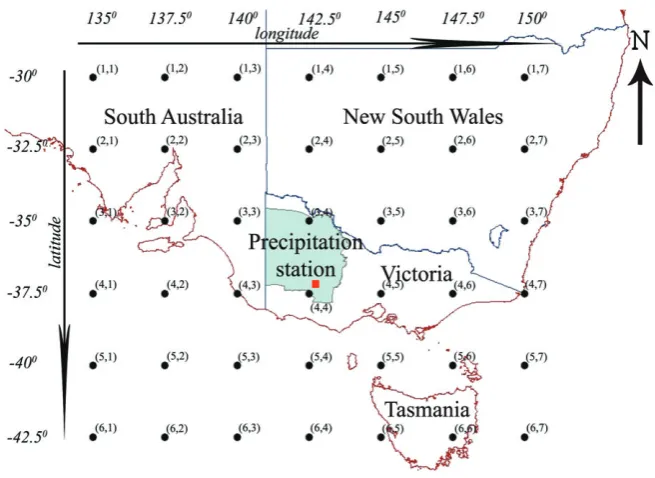
downscaling study. Najafi et al. (2011) successfully used an atmospheric domain with 7×4 grid points in the longitudinal and latitudinal directions, respectively at a spatial resolution of 2.5◦ in both directions, for the statistical downscaling of outputs of CGCM3 to monthly precipitation. Their study demonstrated that the atmospheric domain does not necessarily have to be a square in shape. However, if the atmospheric domain is too rectangular in shape, the influences of large scale atmospheric circulations on the point of interest in the catchment are more considered on the wider sides of the domain, and the influences coming from the narrower sides are less considered or neglected. Hence, such domain shape should be avoided in statistical downscaling. A larger atmospheric domain increases the computational cost and time involved in the investigation. However, a larger domain aids in identifying influences of large scale atmospheric circulations over a wider area. When the atmospheric domain is too small, it may not be able to adequately capture the atmospheric circulations responsible for the hydroclimatology in the catchment. Therefore, the atmospheric domain which is an important component of any statistical downscaling study should be of adequate size and of an appropriate shape. In general a domain size of 6×6 grid points at a spatial resolution of 2.5◦ in both longitudinal and latitudinal directions is a regarded as an adequate size (Tripathi et al., 2006). An atmospheric domain with spatial dimensions of 7×6 grid points at a spatial resolution of 2.5◦ in both longitudinal and latitudinal directions was selected for the downscaling study described in this article. The size of this atmospheric domain was determined considering its ability to represent the large scale atmospheric phenomena which influence the precipitation at the point of interest and also the computational cost. The same atmospheric domain over the same study area was suc-cessfully used by Sachindraet al.(2013) for statistically downscaling GCM outputs to catchment streamflows. The spatial resolution of this atmospheric domain was maintained at 2.5◦ in both longitudinal and latitudinal directions, making it compliant with the spatial resolution of the NCEP/NCAR reanalysis outputs. The atmospheric domain used in this study is shown in Figure 1. The shaded region in Figure 1 depicts the operational area of GWMWater, and the precipitation station considered in this study is located in its south most region.

4.2. Selection of probable and potential predictors for downscaling

(6)

Figure 1. Atmospheric domain for downscaling.

500 hPa, 700 hPa, 850 hPa and 1000 hPa pressure lev-els; relative humidity at 500 hPa, 700 hPa, 850 hPa and 1000 hPa pressure levels; specific humidity at 2 m height, 500 hPa, 850 hPa and 1000 hPa pressure levels; air tem-peratures at 2 m height, 500 hPa, 850 hPa and 1000 hPa pressure levels; surface skin temperature, surface pres-sure, mean sea level prespres-sure, surface precipitation rate and zonal and meridional wind speeds at 850hpa pressure level. These probable predictors were common for all cal-endar months. The monthly data for these 23 probable predictors for the 42 grid points shown in Figure 1 were extracted from the NCEP/NCAR reanalysis data archive at http://www.esrl.noaa.gov/psd/.

The probable predictors and the observed monthly precipitation totals from 1950 to 2010 were split into three 20 year time slices; 1950–1969, 1970–1989 and 1990–2010. The last time slice was 21 years in length. The Pearson correlation coefficients between the probable predictors and the observed monthly precipitation were calculated for all three time slices and the whole period (1950–2010), at each grid point in the atmospheric domain (see Figure 1). The probable predictors which showed good statistically significant correlations (at 95% confidence level, p=0.05) consistently over the three time slices and the whole period were selected as the potential predictors (Sachindraet al., 2013). This process was repeated for all 12 calendar months, yielding 12 sets of potential predictors.

The El Ni˜no-Southern Oscillation (ENSO) and the Indian Ocean Dipole (IOD) are regarded as two large scale atmospheric phenomena influential on the climate of Victoria, Australia. A correlation analysis performed over the period 1950–2010 between the Southern Oscil-lation Index (SOI) which is representative of ENSO and observed precipitation at the Halls Gap post office indi-cated that these correlations vary between 0.03 (March)

and 0.33 (October). Similarly, the correlations between the Dipole Mode Index (DMI) which is representative of IOD and observed precipitation ranged between −0.01 (February) and−0.46 (August) during the period 1958–2010. Hence, it was realized that the influences of these large scale atmospheric phenomena on the observed precipitation at the Halls Gap post office are weak in nature. Therefore it was understood that the inclusion of such indices in the inputs to the downscaling models will not lead to any improvement to the precipitation predic-tions. Furthermore, Chiewet al.(1998) detailed the influ-ences of ENSO on the rainfall, drought and streamflows in Australia, using the SOI and sea surface temperature (SST), and concluded that, the correlations between these ENSO indicators and hydroclimatic variables are not sufficiently strong for a consistent prediction.

4.3. MLR downscaling model calibration and validation

4.3.1. Model calibration and validation with NCEP/NCAR data

(7)

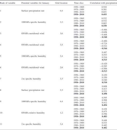
each calendar month the best set of potential predic-tors and the best MLR based downscaling model were selected. Table 1 shows the final (or the best) set of poten-tial predictors used in the downscaling model developed with NCEP/NCAR reanalysis outputs for the month of January. Also this table contains the correlations between the observed precipitation and the final set of potential predictors, during the three 20 year time slices and the whole period of the study.

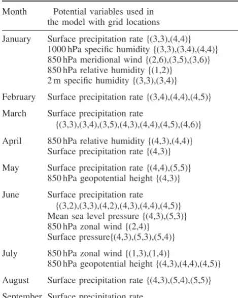
Table 2 provides the final sets of potential predic-tors used in the downscaling models in each calendar month. The final sets of potential predictors used in the downscaling models consisted of: surface precipitation rate; specific humidity, relative humidity and geopoten-tial heights at various pressure levels; mean sea level pressure; surface pressure and zonal and meridional wind speeds at 850 hPa pressure level. However, surface pre-cipitation rate was identified as the most influential poten-tial predictor on precipitation, appearing in the final sets of potential predictors for all calendar months except July. Surface precipitation rate produced by GCMs is a precipitation flux (precipitation per unit time across unit area at earth surface) which is analogous to precipita-tion at a point over a specific time period (e.g. daily or monthly precipitation). Therefore the strong influ-ence of surface precipitation rate on monthly precipita-tion was justified. The highest correlaprecipita-tions between the NCEP/NCAR precipitation rate and the observed precip-itation over the period 1950–2010 within each calendar month were June (0.82), August (0.82), October (0.79), September (0.77), December (0.74), May (0.71), January (0.69), April (0.64), February (0.61), March (0.61) and November (0.48). Precipitation outputs of GCMs have been also used in the past downscaling studies. Tim-bal et al. (2009) used precipitation rate in downscaling daily precipitation and Tisseuilet al.(2010) used precip-itation rate for downscaling daily streamflows. Maraun et al.(2013) stated that despite the errors, the precipita-tion output of a GCM can still contain useful informaprecipita-tion about the observed precipitation. Hence it was realized that precipitation output of a GCM can be used as an input to a downscaling model.

Specific humidity (mass of water vapour per unit mass of air), and relative humidity (ratio of actual water vapour pressure of the air to the saturation vapour pressure) at various pressure levels are indicators of the atmospheric water vapour content which leads to the formation of clouds (Peixoto and Oort, 1996). Humidity variables (relative or specific humidity) which are indictors of the atmospheric water vapour content were potential predictors in 7 (February, March, May, September, October, November and December) of the 12 calendar months. According to Nazemosadat and Cordery (1997), geopotential heights are influential on the generation of precipitation, as they are representative of large scale atmospheric pressure variations such as the El Ni˜no Southern Oscillation (ENSO). Zonal and meridional wind fields are influential on the evaporation from open surface water bodies and they govern the movement

of rain bearing clouds (Bureau of Meteorology, 2010), and hence it was suitable to include wind fields in the final sets of potential predictors. It is noteworthy to mention that, according to Table 2, except in August and November, grid point {4,4} found to be a dominant location for the final sets of potential predictors. The grid point {4,4} is the closest grid point to the precipitation station considered in this study.

In general, humidity variables and precipitation rate are more capable of explaining the precipitation process (refer to Table 2). However as shown in Table 2, in the month of July, the set of potential predictors used in the downscaling models contained only the wind speeds and the geopotential heights at 850 hPa. It was realized that these variables are still able to explain the precipitation process with a good degree of accuracy, as the downscaling model developed for July using the NCEP/NCAR reanalysis outputs displayed NSEs of 0.58 and 0.50 in the calibration and validation phases, respectively. Furthermore, as these potential variables are selected based on the magnitude and also the consistency of correlations with observed precipitation over time, it is argued that the final sets of potential predictors used in the downscaling models are able to characterize the changes in precipitation at the point of interest, also in the future. In Table 2, it could be found that the majority of the potential predictors in the final sets were selected from the grid points surrounding the precipitation station of interest [(3,3), (3,4), (3,5), (4,3), (4,4), (4,5), (5,3), (5,4) and (5,5)]. However, some potential predictors in the final sets were selected from the distant grid points of the domain as the precipitation at the station of interest is not only influenced by the atmosphere in close proximity to the station but also by the atmospheric processes that occur far away. The best grid locations of the potential predictors provided in Table 2 were selected not only based on the strength of the correlation between the potential predictors and observed precipitation, but also considering the consistency of the correlation over three time slices and the whole period of the study. Therefore it was assumed that the best grid locations of the final sets of potential predictors used in this study will remain the same in future.

4.3.2. Model calibration and validation with HadCM3 20th century climate experiment data

(8)

Table 1. Final set of potential predictors used in the January downscaling model and their correlations with observed precipitation in each time slice and whole period.

Rank of variable Potential variables for January Grid location Time slice Correlation with precipitation

1 Surface precipitation rate 4,4

1950–1969 0.910

1970–1989 0.581

1990–2010 0.651

1950–2010 0.693

2 1000 hPa specific humidity 3,3

1950–1969 0.532

1970–1989 0.532

1990–2010 0.603

1950–2010 0.550

3 850 hPa meridional wind 3,6

1950–1969 −0.466

1970–1989 −0.698

1990–2010 −0.468

1950–2010 −0.548

1950–1969 −0.400

1970–1989 −0.724

1990–2010 −0.522

1950–2010 −0.544

1950–1969 0.487

1970–1989 0.553

1990–2010 0.516

1950–2010 0.515

1950–1969 −0.420

1970–1989 −0.585

1990–2010 −0.506

1950–2010 −0.513

7 2 m specific humidity 3,3

1950–1969 0.430

1970–1989 0.550

1990–2010 0.540

1950–2010 0.510

8 Surface precipitation rate 3,3

1950–1969 0.608

1970–1989 0.413

1990–2010 0.523

1950–2010 0.498

1950–1969 0.595

1970–1989 0.508

1990–2010 0.412

1950–2010 0.494

10 850 hPa relative humidity 1,2

1950–1969 0.438

1970–1989 0.475

1990–2010 0.596

1950–2010 0.483

11 2 m specific humidity 3,4

1950–1969 0.448

1970–1989 0.533

1990–2010 0.482

1950–2010 0.482

Bold values refer to calibration and validation periods of the study.

changes in land surface characteristics have been used in HadCM3. The 20th century climate experiment data of HadCM3 were split into two groups; (a) 1950–1989 for model calibration and (b) 1990–1999 for the model validation. HadCM3 data for both the calibration and validation phases were standardized with the means and the standard deviations of HadCM3 data corresponding to 1950–1989 period. In calibration, the standardized sets of data pertaining to the best potential predictors

(9)

Table 2. Final sets of potential predictors for each calendar month.

Month Potential variables used in

the model with grid locations

January Surface precipitation rate{(3,3),(4,4)} 1000 hPa specific humidity{(3,3),(3,4),(4,4)} 850 hPa meridional wind{(2,6),(3,5),(3,6)} 850 hPa relative humidity{(1,2)}

2 m specific humidity{(3,3),(3,4)}

February Surface precipitation rate{(3,4),(4,4),(4,5)}

March Surface precipitation rate

{(3,3),(3,4),(3,5),(4,3),(4,4),(4,5),(4,6)} April 850 hPa relative humidity{(4,3),(4,4)}

Surface precipitation rate{(4,3)} May Surface precipitation rate{(4,4),(5,5)}

850 hPa geopotential height{(4,3)}

June Surface precipitation rate

{(3,2),(3,3),(4,2),(4,3),(4,4),(4,5)} Mean sea level pressure{(4,3),(5,3)} 850 hPa zonal wind{(2,4)}

Surface pressure{(4,3),(5,3),(5,4)} July 850 hPa zonal wind{(1,3),(1,4)}

850 hPa geopotential height{(4,3),(4,4),(4,5)} August Surface precipitation rate{(4,3),(5,4),(5,5)} September Surface precipitation rate

{(2,1),(2,2),(3,2),(3,3),(3,5),(4,2),(4,3),(4,4),(4,5)} 850 hPa relative humidity{(3,3)}

700 hPa relative humidity{(3,4)} October Surface precipitation rate

{(3,2),(4,2),(4,3),(4,4)} 850 hPa relative humidity{(4,3)} 700 hPa geopotential height{(1,1)} November 850 hPa relative humidity{(3,2),(3,3)}

Surface precipitation rate{(4,3),(4,5)} December Surface precipitation rate

{(2,1),(3,2),(4,3),(4,4),(5,5)} 850 hPa relative humidity{(3,2)}

hPa, atmospheric pressure in hectopascal; the locations are given within brackets (see Figure 1).

model which was developed with NCEP/NCAR reanal-ysis outputs, the stepwise development procedure was not adopted in these models. A correlation coefficient analysis performed between the 20th century climate experiment outputs of HadCM3 and NCEP/NCAR reanalysis outputs over the period 1950–1999, revealed that these correlations are quite weak (e.g. 0.2–0.4). Hence it was realized that HadCM3 outputs pertaining to the 20th century climate experiment contain large bias. Therefore it was understood that whether the final sets of potential predictors are selected using a stepwise procedure or not, they will not change the performance of the model developed with HadCM3 outputs. It was assumed that final sets of potential predictors identified in the development of the model driven with NCEP/NCAR outputs are also applicable for this model. The difference

between the statistical downscaling models built with the HadCM3 20th century experiment data (Model(HadCM3))

and the models built with the NCEP/NCAR reanalysis data (Model(NCEP/NCAR)) was that these two models

had different optimum values for their parameters (coefficients and constants in MLR equations).

4.3.3. Calibration and validation results of the downscaling models

Figure 2 shows the time series of monthly observed precipitation and monthly precipitation reproduced by the downscaling model developed with NCEP/NCAR data, for the period 1950–2010. According to Figure 2, the monthly precipitation reproduced by this downscaling model, was in close agreement with the observed pre-cipitation during both calibration and validation periods. Although the model validation was performed in a rela-tively dry period which included the Millennium drought (1997–2010), this downscaling model has been able to capture the monthly precipitation pattern and the magni-tude with good accuracy.

Figure 3 shows the scatter plots of monthly observed precipitation and precipitation reproduced by the down-scaling model developed with NCEP/NCAR data, for the calibration (1950–1989) and validation (1990–2010) phases. As seen in Figure 3, during both the calibration and validation periods, near zero monthly precipitation values were over predicted and relatively large precipita-tion values were under-predicted. However, these scatter plots of the model predictions against the observations further confirmed that, the prediction capabilities of the model developed with NCEP/NCAR data in validation are very much comparable with those during calibration. Figure 4 illustrates the time series of monthly observed precipitation and monthly precipitation reproduced by the downscaling model built with HadCM3 data, for the period 1950–1999. It was seen that this model was not able to satisfactorily reproduce the high precipitation val-ues. Furthermore, the agreement between the observed and model reproduced precipitation was much less com-pared to that of the model developed with NCEP/NCAR reanalysis outputs. However, the model developed with HadCM3 outputs properly captured the pattern of the observed precipitation as shown in Figure 4. It should be noted that the validation phase of the model devel-oped with HadCM3 data was confined to the period 1990–1999, due to the unavailability of data beyond year 1999, under the 20th century climate experiment.

(10)

0 50 100 150 200 250 300 350 400

1950 1951 1952 1953 1954 1955 1956 1957 1958 1959 1960 1961 1962 1963 1964 1965 1966 1967 1968 1969 1970 1971 1972 1973 1974 1975 1976 1977 1978 1979 1980 1981 1982 1983 1984 1985 1986 1987 1988 1989 1990 1991 1992 1993 1994 1995 1996 1997 1998 1999 2000 2001 2002 2003 2004 2005 2006 2007 2008 2009 2010

Observed precipita tion

MLR reproduced precipita tion with NCEP/NCAR data

Pr

ec

ip

it

at

io

n (

m

/m

o

nt

h)

Calibration (1950-1989) Validation (1990-2010)

Figure 2. Observed and Model(NCEP/NCAR)reproduced monthly precipitation (1950 to 2010).

R2_=0.74

0 50 100 150 200 250 300 350

Predicted rainfall (mm/month)

Observed rainfall (mm/month)

0 50 100 150 200 250 300

P

re

d

ic

te

d

ra

in

fa

ll

(mm/mo

n

th

)

(a) Calibration (b) Validation

R2_=0.72

Figure 3. Scatter plots of observed and Model(NCEP/NCAR) reproduced monthly precipitation for calibration (1950–1989) and validation

(1990–2010).

Statistical downscaling models in general fail to cap-ture the full range of the variance of a predictand such as precipitation (Wilby et al., 2004). This is because, in general the variance in the observations of precip-itation is much greater than the variance in the large scale atmospheric variables obtained from the GCM or the reanalysis data. When the downscaling model is run with the GCM or the reanalysis data it tends to explain the mid range of the variance of the observed precip-itation better than the low and high extremes. There-fore statistical downscaling models in general tend to reproduce the average of the precipitation better than the low and high extremes. In other words, this results in an under-estimation of large precipitation values and over-estimations of near zero precipitation values. Tri-pathi et al. (2006) also commented that even a down-scaling model based on support vector machine technique (complex nonlinear regression technique) fails to properly reproduce the extremes of precipitation though it captures the average well.

(11)

0 50 100 150 200 250 300 350 400 19 50 19 51 19 52 19 53 19 54 19 55 19 56 19 57 19 58 19 59 19 60 19 61 19 62 19 63 19 64 19 65 19 66 19 67 19 68 19 69 19 70 19 71 19 72 19 73 19 74 19 75 19 76 19 77 19 78 19 79 19 80 19 81 19 82 19 83 19 84 19 85 19 86 19 87 19 88 19 89 19 90 19 91 19 92 19 93 19 94 19 95 19 96 19 97 19 98 19 99

Observed precipita tion

MLR reproduced precipita tion with Ha dCM3 outputs

P re ci pi ta ti o n ( m m /m ont h)

Calibration (1950-1989) Validation (1990-1999)

Figure 4. Observed and Model(HadCM3)reproduced monthly precipitation (1950 to 1999).

R2_=0.44

0 50 100 150 200 250 300 350

0 50 100 150 200 250 300 350 0 50 100 150 200 250 300

Predicted rainfall (mm/month)

0 50 100 150 200 250 300 P re d ic te d ra in fa ll (mm/mo n th )

R2_=0.22

Figure 5. Scatter plots of observed and Model(HadCM3)reproduced monthly precipitation for calibration (1950–1989) and validation (1990–1999).

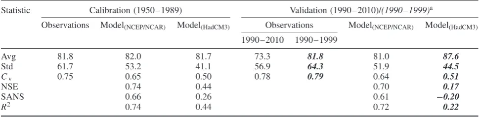
of the observed precipitation. In Figure 4, the same characteristic was seen in the time series plots. This characteristic was seen with less severity in the outputs of the model developed with NCEP/NCAR reanalysis data. The model performances in calibration and validation were further quantified with the NSE, the SANS and the coefficient of determination (R2). The SANS considers the seasonal means of precipitation in measuring the model performances, unlike the original NSE, which con-siders only the mean of precipitation for the whole period. During calibration, the statistical downscaling model developed with NCEP/NCAR reanalysis data displayed NSE, SANS andR2of 0.74, 0.66 and 0.74, respectively. However, for the same period, the downscaling model developed with HadCM3 outputs, produced NSE, SANS and R2 _{of 0.44, 0.26 and 0.44, respectively. In the}

val-idation phase, the model developed with NCEP/NCAR outputs produced NSE, SANS andR2 of 0.70, 0.61 and 0.72. During the validation period, the model developed with HadCM3 outputs, produced NSE, SANS and R2 of 0.17, −0.20 and 0.22, respectively. These findings indicated that both downscaling models have performed

relatively better during the calibration period than in the validation period. However, it was seen that the downscaling model developed with NCEP/NCAR data performed well in the calibration and validation phases, compared to its counterpart model which was built with HadCM3 outputs. This statement was further supported by the findings of scatter plots shown in Figures 3 and 5.

(12)

Table 3. Performances of downscaling models in calibration and validation.

Statistic Calibration (1950–1989) Validation (1990–2010)/(1990–1999)a

Observations Model(NCEP/NCAR) Model(HadCM3) Observations Model(NCEP/NCAR) Model(HadCM3)

1990–2010 1990–1999

Avg 81.8 82.0 81.7 73.3 81.8 81.0 87.6

Std 61.7 53.2 41.1 56.9 64.3 51.9 44.5

Cv 0.75 0.65 0.50 0.78 0.79 0.64 0.51

NSE 0.74 0.44 0.70 0.17

SANS 0.66 0.26 0.61 −0.20

R2 0.74 0.44 0.72 0.22

Avg, average of monthly precipitation in mm;Cv, coefficient of variation; NSE, Nash–Sutcliffe efficiency;R2, coefficient of determination; Std,

standard deviation of monthly precipitation in mm; SANS, Seasonally Adjusted Nash–Sutcliffe efficiency.a_{Bold italicized values in the table}

refer to period 1990–1999.

Figure 7 displays the seasonal scatter plots for the calibration (1950–1989) and validation (1990–1999) periods of the model developed with HadCM3 outputs. Large under-predictions of precipitation were seen in all four seasons during both the calibration and validation phases of this model. During all four seasons in the validation period, a relatively poor agreement between the observed and model reproduced precipitation was seen. This characteristic was more intense in autumn, winter and spring than in summer.

Table 4 shows the seasonal statistics of the observed precipitation and the precipitation reproduced by the models developed with NCEP/NCAR reanalysis and HadCM3 data, for the calibration and validation periods. In the calibration phase, during all four seasons, aver-ages of the observed precipitation were near perfectly reproduced by both downscaling models. In the validation phase, although not as good as in calibration, both mod-els were capable in reproducing the averages of observed precipitation in all four seasons with some under and over-predictions. During all four seasons in the validation period, both downscaling models tended to over-predict the average of the observed precipitation. This was due to the fact that the calibration was performed over a wet-ter period and the validation was done during a relatively dryer period. However, according to Figures 2 and 4 both downscaling models were able to adequately capture the precipitation pattern seen in the observations, through-out the calibration and validation periods. The under-estimation of the standard deviation and the coefficient of variation was seen in all four seasons of both mod-els, during the calibration and validation periods. This characteristic was more severe in the case of the model developed with HadCM3 outputs. Since there is a large scale gap between the GCM outputs and the catchment scale, not all the variance in observations of a predictand (at a point in the catchment) can be explained by the GCM. Therefore, regression based statistical downscal-ing techniques are capable of capturdownscal-ing only the part of the variance (deterministic component of the variance) of a predictand which is conditioned by the GCM (Hewit-son et al., 2013). The local scale random variance of the predictand (stochastic component of the variance) is not

simulated by the regression based downscaling models, as it is not explicitly explained by the GCM. At the catch-ment scale, capturing the full variance of a predictand is important. This can be achieved by the application of a suitable bias-correction method for post-processing the outputs of the downscaling model (Maraun, 2013). Tech-niques such as randomization may also help in capturing the full variance of a predictand (von Storch, 1999).

In the model developed with NCEP/NCAR data, the best performances in calibration in terms of NSE andR2 were seen during winter while the lowest performances were observed in summer. For this model, in validation, autumn produced the best performance. The model devel-oped with HadCM3 outputs showed relatively low NSE and R2_{in all four seasons of the calibration period. The}

negative NSEs were seen in autumn, winter and spring during the validation period, which indicated the limited performances of this downscaling model.

As mentioned in Section 1, the largest drop in pre-cipitation over Victoria during the Millennium drought was observed in autumn. The decline in the average of the observed precipitation in autumn, during the Mil-lennium drought (1997–2010), at the station considered in this study, was 27.5%, from the long-term average (1950–1989). The downscaling model developed with NCEP/NCAR reanalysis outputs was able to successfully reproduce this large drop in the average as 22.4%.

(13)

0 50 100 150 200

0 50 100 150 200 0 50 100 150 200

P re d ic te d p reci pi ta ti on (m m /m ont h)

Observed precipitation (mm/month)

0 50 100 150 200 P red ic te d pr ec ip it at ion ( m m /m o n th)

0 50 100 150 200 250 300 350

P re d ic te d p re cip it at io n (m m/mo n th )

0 50 100 150 200

P re d ic te d p re cip it at io n ( mm/m o n th )

0 50 100 150 200 250 300 350

Pr ed ic te d pr ec ip it at io n (m m /m o nt h)

0 50 100 150 200 250 300

P re d ic te d p reci pi ta ti on (m m /m o nt h)

0 50 100 150 200 250 300

P re d ic te d p re cip it at io n ( m m/ mo n th )

0 50 100 150 200 250

P re d ic te d p re cip it at io n (m m/mo n th )

Summer

Autumn

Winter

Spring

NSE=0.60 / R2_=0.60 _{NSE=0.42 / R}2_=0.45

NSE=0.63 / R2_=0.63 _{NSE=0.75 / R}2_=0.71

NSE=0.70 / R2_=0.70 _{NSE=0.58 / R}2_=0.63

NSE=0.67 / R2_=0.67 _{NSE=0.64 / R}2_=0.65

Figure 6. Seasonal scatter plots of observed and Model(NCEP/NCAR)reproduced monthly precipitation for calibration (1950–1989) and validation

(1990–2010).

was realized that the final sets of potential variables used in the downscaling models are capable of capturing the precipitation process to a good degree.

Figure 8 shows the exceedance probability curve for the observed precipitation, precipitation reproduced by the downscaling models with NCEP/NCAR and HadCM3

(14)

0 50 100 150 200

P re d ic te d p re cip it at io n (mm /mo n th )

0 50 100 150 200

Pr ed ic te d pr ec ip it at io n ( m m /m ont h)

0 50 100 150 200 250 300 350

0 50 100 150 200

0 50 100 150 200 250 300 350

P re d ic te d p re cip it at io n (mm/ mo n th )

0 50 100 150 200 250 300

Pr ed ic te d pr ec ip it at io n (m m /m ont h)

0 50 100 150 200 250 300

P re d ic te d p re cip it at io n (mm/ mo n th )

0 50 100 150 200 250

Summer

Autumn

Winter

Spring

NSE=0.16 / R2_=0.16 _{NSE=0.12 / R}2_=0.13

NSE=0.34 / R2_=0.34 _{NSE= -0.58 / R}2_=0.04

NSE=0.17 / R2_=0.17 _{NSE= -0.20/ R}2_=0.00

NSE=0.32 / R2_=0.32 _{NSE= -0.15/ R}2_=0.09

Figure 7. Seasonal scatter plots of observed and Model(HadCM3) reproduced monthly precipitation for calibration (1950–1989) and validation

(1990–1999).

representative of the precipitation station considered in this study. Note that the precipitation rate (which was the observed precipitation equivalent output of HadCM3) was converted to monthly precipitation, for plotting the corresponding exceedance curve in Figure 8.

(15)

Table 4. Seasonal performances of downscaling models.

Model Statistic Calibration (1950–1989) Validation (1990–2010)/(1990–1999)a

Season Season

Summer Autumn Winter Spring Summer Autumn Winter Spring

Observed

Avg

40.7 73.7 125.1 87.7 42.9/(44.3) 54.1/(57.0) 119.4/(136.1) 78.3/(89.8)

Model(NCEP/NCAR) 40.7 73.7 125.1 87.7 49.2 57.8 132.5 85.1

Model(HadCM3) 40.3 73.8 125.1 87.8 (44.9) (78.8) (128.3) (98.5)

Observed

Std

33.7 58.8 64.5 53.5 41.0/(46.8) 43.1/(46.5) 61.2/(66.3) 48.4/(55.1)

Model(NCEP/NCAR) 26.0 46.6 54.1 43.9 29.8 33.1 54.1 41.7

Model(HadCM3) 15.6 34.4 26.7 30.5 (12.7) (39.0) (30.0) (42.0)

Observed

Cv

0.83 0.80 0.52 0.61 0.96/(1.06) 0.80/(0.82) 0.51/(0.49) 0.62/(0.61)

Model(NCEP/NCAR) 0.64 0.63 0.43 0.50 0.61 0.57 0.41 0.49

Model(HadCM3) 0.39 0.47 0.21 0.35 (0.28) (0.49) (0.23) (0.43)

Model(NCEP/NCAR) _NSE 0.60 0.63 0.70 0.67 0.42 0.75 0.58 0.64

Model(HadCM3) 0.16 0.34 0.17 0.33 (0.12) (−0.58) (−0.20) (−0.15)

Model(NCEP/NCAR) _R2 0.60 0.63 0.70 0.67 0.45 0.71 0.63 0.65

Model(HadCM3) 0.16 0.34 0.17 0.33 (0.13) (0.04) (0.00) (0.09)

Avg, average of monthly precipitation in mm;Cv, coefficient of variation; NSE, Nash–Sutcliffe efficiency;R2, coefficient of determination;

Std, standard deviation of monthly precipitation in mm.a_{Bold italicized values in brackets in the table refer to period 1990–1999.}

0 50 100 150 200 250 300 350

0 0.1 0.2 0.3 0.4 0.5 0.6 0.7 0.8 0.9 1

Observed precipitation 1950-1999

MLR reproduced precipitation with NCEP/NCAR outputs 1950-1999

MLR reproduced precipitation with HadCM3 outputs 1950-1999

20th Century raw precipitation output of HadCM3 at point {4,4} 1950-1999

Exceedance probability

Precipitation /(mm/month)

Figure 8. Precipitation probability exceedance curves (1950–1999).

regional precipitation simulation is less reliable. Larger differences between the observations and raw HadCM3 precipitation outputs were seen for precipitations with low probability of exceedance, such as extremely high precipitations. Furthermore, relatively small anomalies were seen for precipitation values with low magnitudes. For the majority of exceedance probabilities, this mis-match was seen as a large under-prediction in HadCM3 precipitation outputs. The mismatch between the obser-vations and the raw HadCM3 precipitation output was mainly due to the bias present in HadCM3 outputs. As

(16)

have possibly contributed to the bias in the GCM out-puts, as Halls Gap is located in a valley surrounded by a mountain range.

It was noted that the mismatch between the obser-vations and the precipitation downscaled with HadCM3 outputs was less in comparison with that between the observations and the raw precipitation outputs of HadCM3 at grid point {4,4}. This indicated that when the raw outputs of HadCM3 are statistically downscaled to monthly precipitation, the impact of bias in these raw HadCM3 outputs, on downscaled precipitation was less evident. However, this reduction in bias was not adequate as still there was considerable mismatch between the observed and downscaled precipitation (refer to Figure 8). Therefore, it could be argued that a correction to the bias that is present in HadCM3 outputs is needed in producing precipitation projections into future. It was seen that the precipitation exceedance curve of raw precipitation output of HadCM3 at grid point {4,4} had deviated largely from the precipitation exceedance curve of obser-vations. However, the exceedance curves of precipitation reproduced by the downscaling models developed with NCEP/NCAR reanalysis outputs and HadCM3 outputs were in relatively better agreement with the precipitation exceedance curve of observed precipitation. This led to the conclusion that, the precipitation outputs of the downscaling models developed with NCEP/NCAR reanalysis outputs and HadCM3 outputs are much better than the raw precipitation output of HadCM3 at grid point {4,4}. Furthermore, considering the limited agree-ment seen between the precipitation downscaled with the NCEP/NACR and HadCM3 outputs, it was realized that there is a quality mismatch between the data of these two sources. The second article of this series of two companion articles, describes the bias correction and the precipitation projections produced into future in detail.

5. Summary and conclusions

This article, which is the first of a series of two com-panion articles, discussed the development (calibration and validation) of two precipitation downscaling models, employing the MLR technique. The first statistical down-scaling model was developed with the NCEP/NCAR reanalysis outputs and the second downscaling model was developed with the HadCM3 outputs. The precipitation station at the Halls Gap post office which is located in the north western part of Victoria, Australia was selected for the demonstration of the development process of the two downscaling models.

It is the general practice to calibrate and validate the downscaling model with some form of reanalysis data (e.g. NCEP/NCAR) for the past climate, and use the outputs of a GCM pertaining to future on the same downscaling model for the projection of climate into future. The major disadvantage of this procedure is that, for the model development and future projections, data from two entirely different sources are used. This study

investigated the potential of using a downscaling model calibrated and validated with GCM outputs, which does not have the above issue.

The selection of probable predictors for these scaling models was based on the past statistical down-scaling studies and hydrology. Potential predictors were extracted for each calendar month from the set of probable predictors considering the Pearson correlations between the probable predictors and observed precip-itation, under three 20 year time slices (1950–1969, 1970–1989 and 1990–2010) and the entire period of the study (1950–2010). Potential predictors obtained from the NCEP/NCAR reanalysis outputs were introduced to the MLR based downscaling model, sequentially, based on the magnitude of the correlation between observed precipitation and predictors, over the whole period of the study. This process was continued until the model perfor-mances in validation in terms of NSE was maximized. In this manner, the final sets of potential predictors for each calendar month were identified, and downscaling mod-els for each calendar month were developed separately. The HadCM3 outputs corresponding to the final sets of potential predictors identified previously were used for the development of the second downscaling model. It was assumed that these final sets of potential predictors are valid for both downscaling models, developed with NCEP/NCAR and HadCM3 outputs.

The MLR based downscaling model developed with NCEP/NCAR reanalysis outputs proved capable in repro-ducing the observed monthly precipitation during both calibration (1950–1989) and validation (1990–2010) phases. The performances of this model in calibration were slightly better than those in validation. This model was also able to capture the precipitation drop occurred during the Millennium drought (1997–2010) satisfacto-rily. However, it displayed tendencies of over-predicting low precipitation values and under-predicting high pre-cipitation values during both the calibration and valida-tion periods.

(17)

model will reproduce the precipitation during the Millen-nium drought.

The conclusions drawn from this study are:

1. The precipitation rate which is the precipitation equivalent output of a GCM was found as the most influential predictor on precipitation at the station of interest, over the entire year, except in July;

2. Humidity, geopotential heights, mean sea level and surface pressure, and wind speeds also showed good correlations with observed precipitation consistently over time;

3. The downscaling model developed with NCEP/NCAR reanalysis outputs performed well in both calibration and validation, while the per-formances of the model developed with HadCM3 outputs were limited;

4. There was a quality mismatch between the NCEP/NCAR reanalysis and HadCM3 outputs, over the period 1950–1999; and

5. A bias-correction should be applied in projecting the precipitation into future at the station of interest.

The application of the bias-correction and the pro-jections of precipitation into future are presented in the second companion article of this series of articles.

Acknowledgements

The authors acknowledge the financial assistance pro-vided by the Australian Research Council Linkage Grant scheme and the Grampians Wimmera Mallee Water Cor-poration for this project. The authors also wish to thank the editor and the two anonymous reviewers for their use-ful comments, which have improved the quality of this article.

References

Alavian V, Qaddumi HM, Dickson E, Diez SM, Danilenko AV, Hirji RF, Puz G, Pizarro C, Jacobsen M, Blankespoor B. 2009. Water and Climate Change: Understanding the Risks and Making Climate-smart Investment Decisions. The Worldbank: Washington, DC. http://documents.worldbank.org/curated/en/2009/11/11717870/ water-climate-change-understanding-risks-making-climate-smart-investment-decisions (accessed on 19 July 2013).

Anandhi A. 2010. Assessing impact of climate change on season length in Karnataka for IPCC SRES scenarios. J. Earth Syst. Sci. 119: 447–460, DOI: 10.1007/s12040-010-0034-5.

Anandhi A, Srinivas VV, Nanjundiah RS, Kumar DN. 2008. Down-scaling precipitation to river basin in India for IPCC SRES scenarios using support vector machine.Int. J. Climatol.28: 401–420, DOI: 10.1002/joc.1529.

Anandhi A, Srinivas VV, Nanjundiah RS, Kumar DN. 2012. Daily rela-tive humidity projections in an Indian river basin for IPCC SRES sce-narios.Theor. Appl. Climatol.108: 85–104, DOI: 10.1007/s00704-011-0511-z.

Bureau of Meteorology. 2010. Australian Climate Influences. http://www.bom.gov.au/watl/about-weather-and-climate/australian-climate-influences.shtml (accessed 25 September 2012).

Charles A, Timbal B, Fernandez E, Hendon H. 2013. Analog downscal-ing of seasonal rainfall forecasts in the Murray darldownscal-ing basin.Mon. Weather Rev.141: 1099–1117, DOI: 10.1175/MWR-D-12-00098.1.

Chiew FHS, Piechota TC, Dracup JA, McMahon TA. 1998. El Nino/Southern Oscillation and Australian rainfall, streamflow and drought: Links and potential for forecasting. J. Hydrol. 204: 138–149, DOI: 10.1016/S0022-1694(97)00121-2.

Chiew FHS, Young WJ, Cai W, Teng J. 2010. Current drought and future hydroclimate projections in southeast Australia and implications for water resources management.Stoch. Environ. Res. Risk Assess.25: 602–612, DOI: 10.1007/s00477-010-0424-x. Chu JT, Xia J, Xu CY, Singh VP. 2010. Statistical downscaling of daily

mean temperature, pan evaporation and precipitation for climate change scenarios in Haihe River, China.Theor. Appl. Climatol.99: 149–161, DOI: 10.1007/s00704-009-0129-6.

Crowley TJ. 2000. Causes of climate change over the past 1000 years.

Science289: 270–277, DOI: 10.1126/science.289.5477.270. Government of Western Australia Department of Water. 2009.

Streamflow trends in south-west Western Australia. Surface water hydrology series. Report no. HY32. http://www.water.wa.gov.au/ PublicationStore/first/87846.pdf (accessed 1 November 2012). Goyal MK, Burn DH, Ojha CSP. 2012. Evaluation of machine learning

tools as a statistical downscaling tool: temperatures projections for multi-stations for Thames river basin, Canada.Theor. Appl. Climatol. 108: 519–534, DOI: 10.1007/s00704-011-0546-1.

Hashmi MZ, Shamseldin AY, Melville BW. 2011. Statistical down-scaling of watershed precipitation using Gene Expression Pro-gramming (GEP). Environ. Model. Softw. 26: 1639–1646, DOI: 10.1016/j.envsoft.2011.07.007.

Hay LE, Clark MP. 2003. Use of statistically and dynamically downscaled atmospheric model output for hydrologic simulations in three mountainous basins in the western United States.J. Hydrol. 282: 56–75, DOI: 10.1016/S0022-1694(03)00252-X.

Hewitson B, Jack C, Coop L. 2013. Addressing deterministic and stochastic variance in statistical downscaling. InEuropean Geophys-ical Union General Assembly. Vienna, Austria, 7–12 April, 2013. Iizumi T, Takayabu I, Dairaku K, Kusaka H, Nishimori M,

Saku-rai G, Ishizak NN, Adachi SA, Semenov MA. 2012. Future change of daily precipitation indices in Japan: a stochastic weather generator-based bootstrap approach to provide probabilistic cli-mate information.J. Geophys. Res. D: Atmos.117: D11114, DOI: 10.1029/2011JD017197.

IPCC. 2007. IPCC Fourth assessment: synthesis report – summary for policymakers, 6–9. http://www.ipcc.ch/pdf/assessment-report/ ar4/syr/ar4_syr_spm.pdf (accessed on 8 November 2012).

Jeffrey SJ, Carter JO, Moodie KB, Beswick AR. 2001. Using spa-tial interpolation to construct a comprehensive archive of Aus-tralian climate data. Environ. Model. Softw. 16: 309–330, DOI: 10.1016/S1364-8152(01)00008-1.

Kalnay E, Kanamitsu M, Kistler R, Collins W, Deaven D, Gandin L, Iredell M, Saha S, White G, Woollen J, Zhu Y, Chelliah M, Ebisuzaki W, Higgins W, Janowiak J, Mo KC, Ropelewski C, Wang J, Leetmaa A, Reynolds R, Jenne R, Joseph D. 1996. The NCEP/NCAR reanalysis project. Bull. Am. Meteorol. Soc. 77: 437–471, DOI: 10.1175/1520-0477(1996)077<0437:TNYRP>2.0.CO;2.

Kannan S, Ghosh S. 2013. A nonparametric kernel regression model for downscaling multisite daily precipitation in the Mahanadi basin.

Water Resour. Res.49: 1360–1385, DOI: 10.1002/wrcr.20118. Karl TR, Wang WC, Schlesinger ME, Knight RW, Portman D.

1990. A method of relating general circulation model simulated climate to the observed local climate part I: seasonal statis-tics. J. Clim. 3: 1053–1079, DOI: 10.1175/1520-0442(1990)003< 1053:AMORGC>2.0.CO;2.

Khalili M, Brissette F, Leconte R. 2009. Stochastic multi-site gener-ation of daily weather data.Stoch. Environ. Res. Risk Assess. 23: 837–849, DOI: 10.1007/s00477-008-0275-x.

Khazaei MR, Ahmadi S, Saghafian B, Zahabiyoun B. 2013. A new daily weather generator to preserve extremes and low-frequency variability.Clim. Change,DOI: 10.1007/s10584-013-0740-5. Knight J. 2003. Report on forcings for the C20C and EMULATE

HadAM3 experiments. http://hadc20c.metoffice.com/forcings.pdf (accessed on 30 May 2013).

Li H, Sheffield J, Wood EF. 2010. Bias correction of monthly precipitation and temperature fields from Intergovernmental Panel on Climate Change AR4 models using equidistant quantile matching.J. Geophys. Res. D: Atmos.115: 1–20, DOI: 10.1029/2009JD012882. Maraun D. 2013. Bias correction, quantile mapping, and downscal-ing: Revisiting the inflation issue. J. Clim.26: 2137–2143, DOI: 10.1175/JCLI-D-12-00821.1.