Bloom Filters in Adversarial Environments

(1)

Bloom Filters in Adversarial Environments

Moni Naor∗ Eylon Yogev†

Abstract

Many efficient data structures use randomness, allowing them to improve upon deterministic ones. Usually, their efficiency and correctness are analyzed using probabilistic tools under the assumption that the inputs and queries areindependent of the internal randomness of the data structure. In this work, we consider data structures in a more robust model, which we call theadversarial model. Roughly speaking, this model allows an adversary to choose inputs and queries adaptively according to previous responses. Specifically, we consider a data structure known as “Bloom filter” and prove a tight connection between Bloom filters in this model and cryptography.

A Bloom filter represents a setSof elements approximately, by using fewer bits than a precise representation. The price for succinctness is allowing some errors: for anyx∈Sit should always answer ‘Yes’, and for anyx /∈S it should answer ‘Yes’ only with small probability.

In the adversarial model, we consider both efficient adversaries (that run in polynomial time) and computationally unbounded adversaries that are only bounded in the number of queries they can make. For computationally bounded adversaries, we show that non-trivial (memory-wise) Bloom filters exist if and only if one-way functions exist. For unbounded adversaries we show that there exists a Bloom filter for sets of size n and error ε, that is secure against t queries and uses onlyO(nlog1_ε+t) bits of memory. In comparison,nlog1_ε is the best possible under a non-adaptive adversary.

∗

Weizmann Institute of Science. Email: [email protected]. Supported in part by a grant from the I-CORE Program of the Planning and Budgeting Committee, the Israel Science Foundation, BSF and the Israeli Ministry of Science and Technology. Incumbent of the Judith Kleeman Professorial Chair.

†

(2)

1 Introduction

Data structures are one of the most fundamental objects in Computer Science. They provide means to organize a large amount of data such that it can be queried efficiently. In general, constructing efficient data structures is key to designing efficient algorithms. Many efficient data structures use randomness, a resource that allows them to bypass lower bounds on deterministic ones. In these cases, their efficiency and correctness are analyzed in expectation or with high probability.

To analyze randomized data structures, one must first define the underlying model of the analysis. Usually, the model assumes that the inputs (equivalently, the queries) areindependent of the internal randomness of the data structure. That is, the analysis is of the form: For any sequence of inputs, with high probability (or expectation) over its internal randomness, the data structure will yield a correct answer. This model is reasonable in a situation where the adversary picking the inputs gets no information about the internal state of the data structure or about the random bits actually used (in particular, the adversary does not get the responses on previous inputs).1

In this work, we consider data structures in a more robust model, which we call the adversarial model. Roughly speaking, this model allows an adversary to choose inputs and queries adaptively

according to previous responses. That is, the analysis is of the form: With high probability over the internal randomness of the data structure, for any adversary adaptively choosing a sequence of inputs, the response to a single query will be correct. Specifically, we consider a data structure known as “Bloom filter” and prove a tight connection between Bloom filters in this model and cryptography: We show that Bloom filters in an adversarial model exist if and only if one-way functions exist.

Bloom Filters in Adversarial Environments. The approximate set membership problem deals

with succinct representations of a set S of elements from a large universe U, where the price for succinctness is allowing some errors. A data structure solving this problem is required to answer queries in the following manner: for any x∈S it should always answer ‘Yes’, and for anyx /∈S it should answer ‘Yes’ only with small probability. False responses forx /∈S are called false positive

errors.

The study of the approximate set membership problem began with Bloom’s 1970 paper [Blo70], introducing the so-called “Bloom filter”, which provided a simple and elegant solution to the prob-lem. (The term “Bloom filter” may refer to Bloom’s original construction, but we use it to denote any construction solving the problem.) The two major advantages of Bloom filters are: (i) they use significantly less memory (as opposed to storingS precisely) and (ii) they have very fast query time (even constant query time). Over the years, Bloom filters have been found to be extremely useful and practical in various areas. Some primary examples are distributed systems [ZJW04], network-ing [DKSL04], databases [Mul90], spam filtering [YC06,LZ06], web caching [FCAB00], streaming algorithms [NY15,DR06] and security [MW94,ZG08]. For a survey about Bloom filters and their applications see [BM03] and a more recent one [TRL12].

Following Bloom’s original construction many generalizations and variants have been proposed and extensively analyzed, providing better tradeoffs between memory consumption, error probability and running time, see e.g., [CKRT04, PSS09, PPR05, ANS10]. However, as discussed, all known constructions of Bloom filters work under the assumption that the input queryx is fixed, and then the probability of an error occurs over the randomness of the construction. Consider the case where the query results are made public. What happens if an adversary chooses the next query according to

1_{This does not include Las Vegas type data structures, where the output is always correct, and the randomness}

(4)

the responses of previous ones? Does the bound on the error probability still hold? The traditional analysis of Bloom filters is no longer sufficient, and stronger techniques are required.

Let us demonstrate this need with a concrete scenario. Consider a system where a Bloom filter representing a white list of email addresses is used to filter spam mail. When an email message is received, the sender’s address is checked against the Bloom filter, and if the result is negative, it is marked as spam. Addresses not on the white list have only a small probability of being a false positive and thus not marked as spam. In this case, the results of the queries are public, as an attacker might check whether his emails are marked as spam (e.g., spam his personal email account and see if the messages are being filtered). In this case, each query translates to opening a new email account, which might be costly. Moreover, an email address can be easily blocked once abused. Thus, the goal of an attacker is to find a large bulk of email addresses using a small number of queries. Indeed, the attacker, after a short sequence of queries, might be able to find alargebulk of email addresses (much larger than the number of queries) that are not marked as spam although they are not in the white list. Thus, bypassing the security of the system and flooding users with spam mail.

As another example application, Bloom filters are often used for holding the contents of a cache. For instance, a web proxy holds, on a (slow) disk, a cache of locally available web pages. To improve performance, it maintains in (fast) memory a Bloom filter representing all addresses in the cache. When a user queries for a web page, the proxy first checks the Bloom filter to see if the page is available in the cache, and only then does it search for the web page on the disk. A false positive is translates to unsuccessful cache access, that is, a slow disk lookup. In the standard analysis, one would set the error to be small such that cache misses happen very rarely (e.g., one in a thousand requests). However, by timing the results of the proxy, an adversary might learn the responses of the Bloom filter, enabling her to find false positives and cause an unsuccessful cache access for almost every query and, eventually, causing a Denial of Service (DoS) attack. The adversary cannot use a false positive more than once, as after each unsuccessful cache access the web page is added to the cache. These types of attacks are applicable in many different systems where Bloom filters are integrated (e.g., [PKV+14]).

Under the adversarial model, we construct Bloom filters that are resilient to the above attacks. We consider both efficient adversaries (that run in polynomial time) and computationally unbounded adversaries that are only bounded in the number of queries they can make. We define a Bloom filter that maintains its error probability in this setting and say it isadversarial resilient (or just resilient for shorthand).

The security of an adversarial resilient Bloom filter is defined in terms of a game (or an ex-periment) with an adversary. The adversary is allowed to choose the set S, make a sequence of t

adaptive queries to the Bloom filter and get its responses. Note that the adversary has only oracle access to the Bloom filter and cannot see its internal memory representation. Finally, the adversary must output an element x∗ (that was not queried before) which she believes is a false positive. We say that a Bloom filter is (n, t, ε)-adversarial resilient if when initialized over sets of sizenthen after

t queries the probability of x∗ being a false positive is at most ε. If a Bloom filter is resilient t

queries, for any tthat is bounded by a polynomial in nwe say it isstrongly resilient.

(5)

1.1 Our Results

We introduce the notion of adversarial-resilient Bloom filter and show several possibility results (constructions of resilient Bloom filters) and impossibility results (attacks against any Bloom filter) in this context. The precise definitions and the model we consider are given in Section2.

Lower bounds. Our first result is that adversarial-resilient Bloom filters against computationally bounded adversaries that are non-trivial (i.e., they require less space than the amount of space it takes to store the elements explicitly) must use one-way functions. That is, we show that if one-way functions do not exist then any Bloom filter can be ‘attacked’ with high probability.

Theorem 1.1 (Informal). Let B be a non-trivial Bloom filter. If B is strongly resilient against computationally bounded adversaries, then one-way functions exist.

Actually, we show a trade-off between the amount of memory used by the Bloom filter and the number of queries performed by the adversary. Carter et al. [CFG+78] proved a lower bound on the amount of memory required by a Bloom filter. To construct a Bloom filter for sets of size n and error rate εone must use (roughly) nlog1_ε bits of memory (and this is tight). Given a Bloom filter that usesmbits of memory we get a lower bound for its error rateεand thus a lower bound for the (expected) number of false positives. The smaller m is, the larger the number of false positives is, and we prove that the adversary can perform fewer queries.

Bloom filters consist of two algorithms: an initialization algorithm that gets a set and outputs a compressed representation of the set, and a membership query algorithm that gets a representation and an input. Usually, Bloom filters have a randomizedinitialization algorithm but a deterministic

query algorithm that does not change the representation. We say that such Bloom filters have a “steady representation”. However, in some cases, a randomized query algorithm can make the Bloom filter more powerful (see [EPK14] for such an example). Specifically, it might incorporate differentially private [DMNS06] algorithms in order to protect the internal memory from leaking. Differentially private algorithms are designed to protect a private database against adversarial and also adaptive queries from a data analyst. One might hope that such techniques can eliminate the need for one-way functions in order to construct resilient Bloom filters. Therefore, we consider also Bloom filters with “unsteady representation”: where the query algorithm is randomized and

can change the underlying representation on each query. We extend our results (Theorem 1.1) to handle Bloom filters with unsteady representations, which proves that any such approach cannot gain additional security. The proof of the theorem (both the steady and unsteady case) appears in Section4.

Constructions. In the other direction, we show that using one-way functions one can construct a strongly resilient Bloom filter. Actually, we show that one can transform any Bloom filter to be strongly resilient with almost exactly the same memory requirements and at a cost of a single evaluation of a pseudorandom permutation2 (which can be constructed using one-way functions). Specifically, in Section4.4we show:

Theorem 1.2. Let B be an (n, ε)-Bloom filter using m bits of memory. If pseudorandom per-mutations exist, then for security parameter λ there exists a negligible function3 _neg₍_·₎ _{and an}

2

A pseudorandom permutation is family of functions that a random function from the family cannot be distinguished from a truly random permutation by any polynomially bounded adversary making queries to the function. It models a block cipher (See DefinitionA.6).

3_{A function}_neg_:

(6)

(n, ε+neg(λ))-strongly resilient Bloom filter that usesm0 =m+λ bits of memory.

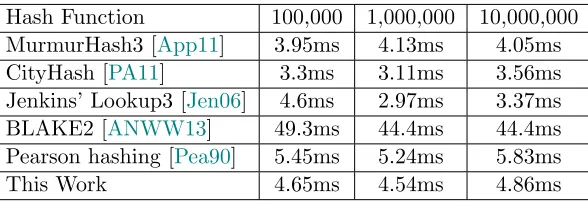
In practice, Bloom filters are used when performance is crucial, and extremely fast implementa-tions are required. This raises implementation difficulties since cryptographically secure funcimplementa-tions rely on relatively heavy computation. Nevertheless, we provide an implementation of an adversarial resilient Bloom filter that is provably secure under the hardness of AES and is essentially as fast as any other implementation of insecure Bloom filters. Our implementation exploits the AES-NI4 instruction set that is embedded in most modern CPUs and provides hardware acceleration of the AES encryption and decryption algorithms [Gue09]. See AppendixBfor more details.

In the context of unbounded adversaries, we show a positive result. For a set of sizenand an error probability of εmost constructions use about O(nlog1_ε) bits of memory. We construct a resilient Bloom filter that does not use one-way functions, is resilient against t queries, uses O(nlog1_ε +t) bits of memory, and has query time O(log1_ε).

Theorem 1.3. There exists an (n, t, ε)-resilient Bloom filter (against unbounded adversaries) for anyn, t∈_N, andε >0 that usesO(nlog1_ε+t) bits of memory and has linear setup time and O(1)

worst-case query time.

1.2 Related Work

One of the first works to consider an adaptive adversary that chooses queries based on the response of the data structure is by Lipton and Naughton [LN93], where adversaries that can measure the

timeof specific operations in a dictionary were addressed. They showed how such adversaries can be used to attack hash tables. Hash tables have some method for dealing with collisions. An adversary that can measure the time of an insert query can determine whether there was a collision and might figure out the precise hash function used. She can then choose the next elements to insert accordingly, increasing the probability of a collision and hurting the overall performance.

Mironov et al. [MNS11] considered the model of sketching in an adversarial environment. The model consists of several honest parties that are interested in computing a joint function in the presence of an adversary. The adversary chooses the inputs of the honest parties based on the shared random string. These inputs are provided to the parties in an on-line manner, and each party incrementally updates a compressed sketch of its input. The parties are not allowed to communicate, they do not share any secret information, and any public information they share is known to the adversary in advance. Then, the parties engage in a protocol in order to evaluate the function on their current inputs using only the compressed sketches. Mironov et al. construct explicit and efficient (optimal) protocols for two fundamental problems: testing equality of two data sets and approximating the size of their symmetric difference.

In a more recent work, Hardt and Woodruff [HW13] considered linear sketch algorithms in a similar setting. They consider an adversary that can adaptively choose the inputs according to previous evaluations of the sketch. They ask whether linear sketches can be robust to adaptively chosen inputs. Their results are negative: They showed that no linear sketch approximates the Eu-clidean norm of its input to within an arbitrary multiplicative approximation factor on a polynomial number of adaptively chosen inputs.

One may consider adversarial resilient Bloom filters in the framework of computational learning theory. The task of the adversary is to learn the private memory of the Bloom filter in the sense that it is able to predict on which elements the Bloom filter outputs a false positive. The connection between learning and cryptographic assumptions has been explored before (already in his 1984

(7)

paper introducing the PAC model Valiant’s observed that the nascent pseudorandom functions imply hardness of learning [Val84]). In particular, Blum et al. [BFKL93] showed how to construct several cryptographic primitives (pseudorandom bit generators, one-way functions and private-key cryptosystems) based on certain assumptions on the difficulty of learning. The necessity of one-way functions for several cryptographic primitives has been shown in [IL89].

2 Model and Problem Definitions

In our model, we are given a universe U = [u] of elements, and a subset S ⊂ U of size n. For simplicity of presentation, we consider mostly the static problem, where the set is fixed throughout the lifetime of the data structure. In the dynamic setting, the Bloom filter is initially empty, and the user can add elements to the set in between queries. We note that the lower bounds imply the same bounds for the dynamic case and the cryptographic upper bound (Theorem 4.1) actually works in the dynamic case as well.

A Bloom filter is a data structure B= (B1,B2) composed of a setup algorithm B1 (or “build”)

and a query algorithm B2 (or “query”). The setup algorithm B1 is randomized, gets as input a

set S, and outputs B1(S) = M which is a compressed representation of the set S. To denote the

representationM on a setSwith random stringrwe writeB1(S;r) =MrS; its size in bits is denoted

as|M_rS|.

The query algorithm answers membership queries to S given the compressed representationM. That is, it gets an inputxfromU and answers with 0 or 1. (The idea is that the answer is 1 only if

x∈S, but there may be errors.) Usually, in the literature, the query algorithm is deterministic and cannot change the representation. In this case, we sayB has a steady representation. However, we also consider Bloom filters where their query algorithm israndomized and can change the represen-tation M after each query. In this case, we say that B has an unsteady representation. We define both variants.

Definition 2.1 (Steady-representation Bloom filter). Let B = (B1,B2) be a pair of

polynomial-time algorithms where B1 is a randomized algorithm that gets as input a set S and outputs a

representation, andB2 is a deterministic algorithm that gets as input a representation and a query

elementx∈U. We say thatB is an (n, ε)-Bloom filter (with a steady representation) if for all sets

S of size nin a suitable universe U it holds that:

1. Completeness: For anyx∈S: Pr[B2(B1(S), x) = 1] = 1

2. Soundness: For any x /∈S: Pr[B2(B1(S), x) = 1]≤ε,

where the probabilities are over the setup algorithmB1.

False Positive and Error Rate. Given a representationM of S, ifx /∈S and B2(M, x) = 1 we

say thatxis afalse positive with respect toM. Moreover, ifBis an (n, ε)-Bloom filter then we say thatB haserror rate at mostε.

Definition2.1considers only a single fixed inputxand the probability is taken over the random-ness of B. We want to give a stronger soundness requirement that considers a sequence of inputs

x1, x2, . . . , xtthat is not fixed but chosen by an adversary, where the adversary gets the responses of

(8)

responsible for choosing a setS. Then,A2 getS as input, and its goal is to find a false positivex∗,

given only oracle access to a Bloom filter initialized withS. The adversary A succeeds if x∗ is not among the queried elements and is a false positive. We measure the success probability of A with respect to the randomness in B1 and inA.

Note that in this case, the setup phase of the Bloom filter and the adversary get an additional input, which is the numberλ(given in unary as 1λ). This is called thesecurity parameter. Intuitively, this is like the length of a password, that is, as it increases the security gets stronger. More formally, it enables the running time of the Bloom filter to be polynomial inλand thus the errorε=ε(λ) can be a function of λ. From here on, we always assume that B has this format, however, sometimes we omit this additional parameter from the writing when clear from the context. For a steady representation Bloom filter we define:

Definition 2.2 (Adversarial-resilient Bloom filter with a steady representation). LetB= (B1,B2)

be an (n, ε)-Bloom filter with a steady representation (see Definition 2.1). We say that B is an (n, t, ε)-adversarial resilient Bloom filter (with a steady representation) if for any probabilistic polynomial-time adversaryA= (A1, A2) for all large enoughλ∈Nit holds that:

• Adversarial Resilient: Pr[Challenge_A,t(λ) = 1]≤ε,

where the probabilities are taken over the internal randomness of B1 and A. The random variable Challenge_A,t(λ) is the outcome of the following algorithm (see also Figure 1):

Challenge_A,t(λ):

1. S←A1(1λ+nlogu) whereS ⊂U, and |S|=n.

2. M ←B1(1λ+nlogu, S).

3. x∗ ←AB2(M,·)

2 (1λ+nlogu, S) whereA2performs at mosttadaptive queriesx1, . . . , xttoB2(M,·).

4. Ifx∗∈/ S∪ {x1, . . . , xt}and B2(M, x∗) = 1 output 1, otherwise output 0.

2

𝑆

𝑀 ← 𝐵

1

𝑆

𝑥

𝑖

Challenger

Adversary

𝑦

𝑖

← 𝐵

2

𝑀, 𝑥

𝑖

𝑦

𝑖

𝑥

∗

𝑦

∗

_{← 𝐵}

2

(𝑀, 𝑥

∗

)

𝑡

(9)

Unsteady representations. When the Bloom filter has an unsteady representation, then the algorithmB2 is randomized and moreover can change the representationM. That is,B2 is a query

algorithm that outputs the response to the query as well as a new representation. That is, the data structure has an internal state that might be changed with each query and the user can perform queries to this data structure. Thus, the user or the adversary do not interact directly withB2(M,·)

but with an interface Q(·) (initialized with some M∗) that on query x updates its representation

M and outputs only the response to the query (i.e., it cannot issue successive queries to the same memory representation but to one that keeps changing). Formally, Q(·) is with M∗ and at each point in time has a memoryM. Then, on inputx is acts as follows:

The interface Q(x):

1. (M0, y)←B2(M, x).

2. M ←M0.

3. Outputy.

We define a variant of the above interface, denoted by Q(x;x1, . . . , xt) (initialized with M∗) as

first performing the queriesx1, . . . , xt and then performing the queryx and output the result onx.

Formally, we define:

Q(x;x1, . . . , xt):

1. Fori= 1. . . tqueryQ(xi).

2. OutputQ(x).

We define an analog of the original Bloom filter for unsteady representations and then define an adversarial resilient one.

Definition 2.3 (Bloom filter with an unsteady representation). Let B = (B1,B2) be a pair of

probabilistic polynomial-time algorithms such thatB1 gets as input the setS of sizenand outputs

a representationM0, and B2 gets as input a representation and query x and outputs a new

repre-sentation and a response to the query. Let Q(·) be the process initialized withM0. We say that B

is an (n, ε)-Bloom filter (with an unsteady representation) if for any such set S the following two conditions hold:

1. Completeness: For any x∈S, for anyt∈_Nand for any sequence of queries x1, x2, . . . , xt we

have that Pr[Q(x;x1, . . . , xt) = 1] = 1.

2. Soundness: For anyx /∈S, for anyt∈_Nand for any sequence of queriesx1, x2, . . . , xtwe have

that Pr[Q(x;x1, . . . , xt) = 1]≤ε,

where the probabilities are taken over the internal randomness of Q.

The above definition is for fixed query sequences, where the next definition is for adaptively chosen query sequences.

Definition 2.4 (Adversarial-resilient Bloom filter with an unsteady representation). Let B = (B1,B2) be an (n, ε)-Bloom filter with an unsteady representation (see Definition 2.3). We say

(10)

• Adversarial Resilient: Pr[Challenge_A,t(λ) = 1]≤ε,

where the probabilities are taken over the internal randomness of B1,B2 and A and where the

random variableChallenge_A,t(λ) is the outcome of the following process:

Challenge_A,t(λ):

1. S←A1(1λ+nlogu) whereS ⊂U, and |S| ≤n.

2. M0←B1(S,1λ+nlogu).

3. Initialize Q(·) with M0.

4. x∗ ←AQ₂(·)(1λ+nlogu, S) whereA2 performs at mostt adaptive queriesx1, . . . , xt toQ(·).

5. Ifx∗∈/ S∪ {x1, . . . , xt}and Q(x∗) = 1 output 1, otherwise output 0.

If B is not (n, t, ε)-resilient then we say there exists an adversary A that can (n, t, ε)-attack B. IfB is resilient for any polynomial number of queries we say it isstrongly resilient:

Definition 2.5 (Strongly resilient). For a security parameterλ, we say thatB is an (n, ε)-strongly resilient Bloom filter, if for any polynomial t = t(λ, n) it holds that B is an (n, t, ε)-adversarial resilient Bloom filter.

Remark 2.6 (Access to the setS). Notice that in Definitions 2.2and 2.4the adversaryA1 chooses

the set S, and then the adversary A2 gets the set S as an additional input. This strengthens the

definition of the resilient Bloom filter such that even given the setS it is hard to find false positives. An alternative definition might be to not give the adversary A2 the set. However, our results of

Theorem1.1hold even if the adversary does not get the set. That is, the algorithm that predicts a false positive makes no use of the set S. Moreover, the construction in Theorem1.2 holds in both cases, even against adversaries that do get the set.

An important parameter is the memory use of a Bloom filter B. We sayB uses m=m(n, λ, ε) bits of memory if for any setS of sizenthe largest representation is of size at most m. The desired properties of Bloom filters is to have m as small as possible and to answer membership queries as fast as possible. LetB be a (n, ε)-Bloom filter that uses m bits of memory. Carter et al. [CFG+78] (see also [DP08] for further details) proved a lower bound on the memory use of any Bloom filter showing that if u > n2/ε thenm ≥nlog1_ε (or written equivalently as ε≥2−mn). This leads us to

define the minimal error of B.

Definition 2.7 (Minimal error). LetB be an (n, ε)-Bloom filter that uses m bits of memory. We say that ε0 = 2−

m

n is the minimal error ofB.

Note that using the lower bound of [CFG+78] we get that for any (n, ε)-Bloom filter its minimal errorε0 always satisfies ε0 ≤ε. For technical reasons, we will have a slightly different condition on

the size of the universe, and we require that u = Ω(m/ε2₀). Moreover, if u is super-polynomial in

n, andεis negligible in nthen any polynomial-time adversary has only negligible chance in finding any false positive, and again we say that the Bloom filter is trivial.

Definition 2.8 (Non-trivial Bloom filter). Let B be an (n, ε)-Bloom filter that uses m bits of memory and let ε0 be the minimal error of B (see Definition 2.7). We say that B is non-trivial if

for all constantsa >0 it holds thatu > a_ε·m2 0

(11)

3 Our Techniques

3.1 One-Way Functions and Adversarial Resilient Bloom Filters

We present the main ideas and techniques of the equivalence of adversarial resilient Bloom filters and one-way functions (i.e., the proof of Theorems 1.1 and 1.2). The simpler direction is showing that the existence of one-way functions implies the existence of adversarial resilient Bloom filters. Actually, we show that any Bloom filter can be efficiently transformed to be adversarial resilient with essentially the same amount of memory. The idea is simple and works in general for other data structures as well: apply a pseudo-random permutation of the input and then send it to the original Bloom filter. The point is that an adversary has almost no advantage in choosing the inputs adaptively, as they are all randomized by the permutation, while the correctness properties remain under the permutation.

The other direction is more challenging. We show that if one-way functions do not exist then any non-trivial Bloom filter can be “attacked” by an efficient adversary. That is, the adversary performs a sequence of queries and then outputs an elementx∗ (that was not queried before) which is a false positive with high probability. We give two proofs: One for the case where the Bloom filter has a steady representation and one for an unsteady representation.

The main idea is that although we are given only oracle access to the Bloom filter, we are able to construct an (approximate) simulation of it. We use techniques from machine learning to (efficiently) ‘learn’ the internal memory of the Bloom filter, and construct the simulation. The learning task for steady and unsteady Bloom filters is quite different and each yield a simulation with different guarantees. Then we show how to exploit each simulation to find false positives without querying the real Bloom filter.

In the steady case, we state the learning process as a ‘PAC learning’ [Val84] problem. We use what’s known as ‘Occam’s Razor’ which states that any hypothesis consistent on a large enough random training set will have a small error. Finally, we show that since we assume that one-way functions do not exist, we are able to find a consistent hypothesis in polynomial time. Since the error is small, the set of false positive elements defined by the real Bloom filter is approximately the same set of false positive elements defined by the simulator.

Handling Bloom filters with an unsteady representation is much more complex. Recall that such Bloom filters are allowed to randomly change their internal representation after each query. In this case, we are trying to learn a distribution that might change after each sample. We describe two examples of Bloom filters with unsteady representations which seem to capture the main difficulties of the unsteady case.

The first example considers any ordinary Bloom filter with error rateε/2, where we modify the query algorithm to first answer ‘1’ with probability ε/2 and otherwise continue with its original behavior. The resulting Bloom filter has an error rate of ε. However, its behavior is tricky: When observing its responses, elements can alternate between being false positive and negatives, which makes the learning task much harder.

The second example consists of two ordinary Bloom filters with error rateε, both initialized with the setS. At the beginning, only the first Bloom filter is used, and after a number of queries (which may be chosen randomly) only the second one is used. Thus, when switching to the second Bloom filter the set of false positives changes completely. Notice that while first Bloom filter was used exclusively, no information was leaked about the second. This example proves that any algorithm trying to ‘learn’ the memory of the Bloom filter cannot perform a fixed number of samples (as does our learning algorithm for the steady representation case).

(12)

presented by Naor and Rothblum [NR06], which models the task of learning distributions that can adaptively change after each sample was studied. Their main result is that if one-way functions do not exist then there exists an efficient learning algorithm that can approximate the next activation of the ACD, that is, produce a distribution that is statistically close to the distribution of the next activation of the ACD. We show how to facilitate (a slightly modified version of) this algorithm to learn the unsteady Bloom filter and construct a simulation. One of the main difficulties is that since we get only a statistical distance guarantee, a false positive for the simulation need not be a false positive for the real Bloom filter. Nevertheless, we show how to estimate whether an element is a false positive in the real Bloom filter.

3.2 Computationally Unbounded Adversaries

In Theorem1.3 we construct a Bloom Filter that is resilient against any unbounded adversary for a given number (t) of queries. One immediate solution would be to imitate the construction of the computationally bounded case while replacing the pseudo-random permutation with ak= (t+n )-wise independent hash function. Then, any set of t queries along with the n elements of the set would behave as truly random under the hash function. The problem with this approach is that the representation of the hash function is too large: It is O(klog|U|) which is more than the number of bits needed for a precise representation of the set S. Turning to almost k-wise independence does not help either. First, the memory will still be too large (it can be reduced to

O(nlognlog1_ε +tlognlog1_ε) bits) and second, we get that only sets chosen in advance will act as random, where the point of an adversarial resilient Bloom filter is to handle adaptively chosen sets. Carter et al. [CFG+78] presented a general transformation from any exact dictionary to a Bloom filter. The idea was simple: storingx in the Bloom filter translates to storingg(x) in a dictionary for some (universal) hash function g : U → V, where |V| = n_ε. The choice of the hash function and underlying dictionary are important as they determine the performance and memory size of the Bloom filter. Notice that, at this point replacing g with a k = (t+n)-wise independent hash function (or an almost k-independent hash function) yields the same problems discussed above. Nevertheless, this is the starting point for the construction, and we show how to overcome these issues. Specifically, we combine two main ingredients: Cuckoo hashing and a highly independent hash function tailored for this construction.

For the underlying dictionary in the transformation, we use the Cuckoo hashing construction [PR04,Pag08]. Using cuckoo hashing as the underlying dictionary was already shown to yield good constructions for Bloom filters by Pagh et al. [PPR05] and Arbitman et al. [ANS10]. Among the many advantages of Cuckoo hashing (e.g., succinct memory representation, constant lookup time) is the simplicity of its structure. It consists of two tablesT1 and T2 and two hash functions h1 and

h2 and each elementx in the Cuckoo dictionary resides in eitherT1[h1(x)] orT2[h2(x)]. However,

we use this structure a bit differently. Instead of storing g(x) in the dictionary directly (as the reduction of Carter et al. suggests) which would resolve to storing g(x) at either T1[h1(g(x))] or

T2[h2(g(x))] we storeg(x) at eitherT1[h1(x)] or T2[h2(x)]. That is, we use the full description of x

to decide wherexis stored but eventually store only a hash ofx(namely,g(x)). Since each element is compared only with two cells, we can reduce the size ofV toO 1_ε (instead of n_ε).

(13)

range of the function).

Note that the guarantee of the function acting randomly holds only for sets S of sizek that are

chosen in advance. In our case, the set is not chosen in advance but rather chosen adaptively and adversarially. However, Berman et al. [BHKN13] showed that the construction of Pagh and Pagh still workseven when the set of queries is chosen adaptively.

At this point, one solution would be to use the family of functions Gsettingk=t+n, with the analysis of Berman et al. as the hash functiongand the structure of the Cuckoo hashing dictionary. To get an error of ε, we set |V| = O log1_ε

and get an adversarial resilient Bloom filter that is resilient for t queries and uses O nlog1_ε +tlog1_ε bits of memory. However, our goal is to get a memory size of O nlog1_ε +t.

To reduce the memory of the Bloom filter even further, we use the family G a bit differently. Let ` = O log1_ε, and set k = O(t/`). We define the function g to be a concatenation of `

independent instancesgi of functions fromG, each outputting a single bit (V ={0,1}). Using the

analysis of Berman et al. we get that each of them behaves like a truly random function for any sequence of kadaptively chosen elements. Consider an adversary performing tqueries. To see how this composition of hash functions helps reduce the independence needed, consider the comparisons performed in a query between g(x) and some value y being performed bit by bit. Only if the first pair of bits are equal we continue to compare the next pair. The next query continues from the last pair compared, in a cyclic order. For any set of k elements, the probability of the two bits to be equal is 1/2. Thus, with high probability, only a constant number of bits will be compared during a single query. That is, in each query only a constant number of function gi will be involved and

“pay” in their independence, where the rest remain untouched. Altogether, we get that although there are t queries performed, we have ` different functions and each function gi is involved in at

mostO(t/`) =k queries (with high probability). Thus, the view of each function remains random on these elements. This results in an adversarial resilient Bloom filter that is resilient for tqueries and uses onlyO(nlog1_ε +klog1_ε) =O(nlog1_ε+t) bits of memory.

4 Adversarial Resilient Bloom Filters and One-Way Functions

In this section, we show that adversarial resilient Bloom filters are (existentially) equivalent to one-way functions (see Definition A.1). We begin by showing that if one-way functions do not exist, then any Bloom filter can be “attacked” by an efficient algorithm in a strong sense:

Theorem 4.1. Let B = (B1,B2) be any non-trivial Bloom filter (possibly with unsteady repre-sentation) of n elements that uses m bits of memory and let ε0 be the minimal error of B.5 If one-way functions do not exist, then for any constant ε <1, B is not (n, t, ε)-adversarial resilient for t=O m/ε2₀

.

We give two different proofs; The first is self-contained (in particular, we do use the Impagliazzo-Luby [IL89] technique of finding a random inverse), but, deals only with Bloom filters with steady representations. The second handles Bloom filters with unsteady representations, and uses the framework of adaptively changing distributions of [NR06].

4.1 A Proof for Bloom Filters with Steady Representations.

Overview: We prove Theorem4.1for Bloom filters with steady representation (see Definition2.1). Actually, for the steady case the theorem holds even fort=O(m/ε0). In both cases, the adversary

5_{The definition of non-trivial is according to Definition}_2.8_{. The definition of stead and unsteady representations}

(14)

A1 chooses a uniformly random setS. Thus, we focus on describing the adversaryA2.

Assume that there are no one-way functions. We want to construct an adversary that can attack the Bloom filter. We define a function f to be a function that gets a set S, random bits r, and elements x1, . . . , xt, computesM =B1(S;r) and outputs x1, . . . , xt along with their evaluation on B2(M,·) (i.e. for each element xi the valueB2(M, xi)). Sincef is not one-way, there is an efficient

algorithm that can invert it with high probability6. That is, the algorithm is given a random set of elements labeled with the information whether they are (false) positives or not and it outputs a set S0 and bits r0. For M0 =B1(S0;r0) the functionB2(M0,·) is consistent withB2(M,·) for all

the elements x1, . . . , xt. For a large enough set of queries we show thatB2(M0,·) is actually a good

approximation of B2(M,·) as a function fromU to{0,1}.

We useB2(M0,·) to find an inputx∗6∈Ssuch thatB2(M0, x∗) = 1 and show thatB2(M, x∗) = 1

as well (with high probability). This contradicts B being adversarial-resilient and proves that f is a (weak) one-way function (see DefinitionA.2).

Proof of Theorem 4.1(for the steady case). LetB= (B1,B2) be an adversarial-resilient Bloom filter

(see Definition 2.2) that uses m bits of memory, initialized with a random set S of size n, and let

M = B1(S) be its representation. Assume that one-way functions do not exist. Our goal is to

construct an algorithm that, given access to B2(M,·), finds an element x∗ ∈/ S that is a false

positive with probability greater than ε. For the simplicity of presentation, we assume ε≤2/3 (for other values of ε the same proof works while adjusting the constants appropriately). We need to show an attack on infinitely many n’s, and thus throughout the proof we assume thatn andm are large enough. We describe the function f (which we intend to invert).

The Function f. The function f takes N = log u_n+r(n) +tlogu bits as inputs where r(n) is the number of random coins thatB1 uses (r(n) is polynomial sinceB1runs in polynomial time) and

t= 200_εm

0 . The function f uses the first log u n

bits to sample a set S of size n, the next r(n) bits (denoted byr) are used to runB1 onS and getMrS =B1(S;r). The lasttlogubits are interpreted

as telements of U denoted x1, . . . , xt. The output off is a sequence of these elements along with

their evaluation byB2(MrS,·). Formally, the definition of f is:

f(S, r, x1, . . . , xt) =x1, . . . , xt,B2(MrS, x1), . . . ,B2(MrS, xt)

whereM_rS =B1(S;r).

It is easy to see that f is polynomial-time computable. Moreover, we can obtain the output of

f on a uniform input by sampling x1, . . . , xt and querying the oracle B2(M,·) on these elements.

As shown before (see [Gol01] Section 2.3), if one-way functions do not exist then weak one-way functions (see Definition A.2) also do not exist. Thus, we can assume that f is not weakly one-way. In particular, we know that there exists a polynomial-time algorithm A that inverts f with probability at least 1−1/100. That is:

Pr[f(A(f(S, r, x1, . . . , xt))) =f(S, r, x1, . . . , xt)]≥1−1/100.

Using A we construct an algorithm Attack that will find a false positive x∗ using t queries with probability 2/3. The description of the algorithm is given in Figure 2.

We need to show that the success probability of Attack is more than 2/3. That is, if x∗ is the output of theAttack algorithm then we want to show that Pr[B2(M, x∗) = 1]≥2/3. Our first step

is showing that if A successfully inverts f then with high probability the resulting M0 defines a

6_{The algorithm can invert the function for infinitely many input sizes. Thus, the adversary we construct will}

(15)

The Algorithm Attack

Given: Oracle access to the query algorithmB2(M,·). The setS. Input: 1λ_{, n, m, u}_.

1. Fori∈[t] samplexi∈U uniformly at random and queryyi=B2(M, xi).

2. Run A(the inverter off) on (x1, . . . , xt, y1, . . . , yt) and 1λ to get an inverse (S0, r0, x1, . . . , xt).

3. ComputeM0=B1(S0;r0).

4. Dok= 200_ε

0 times:

(a) Samplex∗_∈_U_{\ {x}

1, . . . , xt} ∪S uniformly at random.

(b) IfB2(M0, x∗) = 1 outputx∗ and HALT.

5. Output an arbitraryx∗_∈_U_.

Figure 2: The description of the algorithmAttack.

function that agrees with B2(M,·) on almost all points. For any representationsM, M0 define their

error by:

err(M, M0) := Pr

x∈U[B2(M, x)6=B2(M

0_{, x}_)]_,

where x is chosen uniformly at random from U. Using this notation we prove the following claim which is very similar to what is known as “Occam’s Razor” in learning theory [BEHW89].

Claim 4.2. Let t= 1000_ε m

0 . Then, for any representationM, over the random choices of x1, . . . , xt,

the probability that there exists a representation M0 that is consistent with M (i.e., that for i∈[t],

B2(M, xi) =B2(M0, xi)) and err(M, M0)> ₁₀₀ε0 is at most 1/100.

Proof. Fix M and consider any M0 such that err(M, M0) > ε0/100. We want to bound from

above the probability over the choice of xi’s thatM0 is consistent with M on x1, . . . , xt. From the

independence of the choice of the xi’s we get that

Pr

x1,...,xt

∀i∈[t] :B2(M, xi) =B2(M0, xi)

≤1− ε0

100

t .

Since the data structure uses m bits of memory, there are at most 2m possible representations and at most 2m candidates for M0. Taking a union bound over the all candidates and for t= 800_εm

0 we

get that the probability that there exists such a M0 is:

Pr

x1,...,xt

∃M0:∀i∈[t],B2(M, xi) =B2(M0, xi)

≤2m

1− ε0

100

t

≤2m·e−10m ≤ 1

100.

By the definition of f, if A successfully inverts f then it must output S0 and r0 such that M0 =

B1(S0;r0) is a representation that is consistent withM on all samplesx1, . . . , xt. Thus, assumingA

inverts successfully we get that the probability thaterr(M, M0)> ε0/100 is at most 1/100.

Given that err(M, M0) ≤ ε0/100, we want to show that with high probability step 4 will halt

(16)

of M. The number of false positives might depend onS. For instance, a Bloom filter might store the setS precisely if S is some special set fixed in advance, and thenµ(M) =n. However, we show that for most sets the fraction of positives must be approximatelyε0.

Claim 4.3. For any Bloom filter with minimal errorε0 it holds that:

Pr

S

h

∃r:µ M_rS≤ ε0

8

i

≤2−n

where the probability is taken over a uniform choice of a set S of size nfrom the universe U.

Proof. LetBADbe the set of all setsS such that there exists anr such that µ(M_rS)≤ ε0

8. Since the

number of sets S is u_n, we need to show that |BAD| ≤ 2−n u_n. We show this using an encoding argument for S. Given S ∈ BAD there is an r such that µ(M_rS) ≤ ε0

8. Let Sb be the set of all

elements x such that B2(MrS, x) = 1. Then,|Sb| ≤ ε0₈u, and we can encode the set S relative to Sb

using the representation M_rS: EncodeM_rS and then specify S from all subsets of Sb of size n. This

encoding must be more than log|BAD|bits and hence we get the bound:

log|BAD| ≤m+ log

ε0u/8

n

≤m+nlog (ε0u/8)−nlogn+ 2n≤ −n+ log

u n

,

where the second inequality follows from LemmaA.8.

Assuming that M0 is an approximation of M, it follows that µ(M0) ≈ µ(M), and therefore in step 4 with high probability we will find an x∗ such that B2(M, x∗) = 1. Namely, we get the

following claim.

Claim 4.4. Assume that err(M, M0) ≤ ε0/100 and that µ(M) ≥ ε0/8. Then, with probability at least 1−1/100 the algorithm Attack will halt on step 4, where the probability is taken over the internal randomness of Attack and over the random choices of x1, . . . , xt.

Proof. Recall that B is non-trivial and by definition, we have that ε0 > am/u (for any constant

a) and that there exists a constant c ≥ 1 such that ε > 1/nc. Since err(M0, M) ≤ ε0/100 and

µ(M)≥ε0/8 we get that

µ(M0)≥ ε0

8 −

ε0

100 >

ε0

10.

Let Sb0 = {x : B₂(M0, x) = 1} be the set of positives (false and true) relative to M0. Let X =

{x1, . . . , xt} be a multiset of the t elements sampled by the algorithm. The probability of each

element to be sampled fromSb0 isµ(M0), and thus the expectation is:

E h

|Sb0∩ X | i

=t·µ(M0)≥ 1000m

ε0 · ε0

10 = 100m.

By a Chernoff bound we get that:

Pr

h

|Sb0∩ X |<200m i

>1−e−Ω(m).

Thus, choosing a large enough constanta we get that

|Sb0\(X ∪S)| ≥ |Sb0| − |Sb0∩ X | − |S| ≥u·µ(M0)−200m−n≥ uε0

(17)

Thus, we can bound the probability of sampling a successfulx∗

Pr

x∗_∈_U_\{_x

1,...,xt}∪S

[x∗∈Sb0]≥

|Sb0\(X ∪S)|

u ≥

ε0

10 − 200m

u −n/u≥ ε0

10 −

ε0

20 =

ε0

20,

where the last inequality holds since u > am_ε

0 for any constant a > 0. That is, the probability of

failing is at most 1−ε0/20 and thus the probability of failing in all k= 100_ε₀ attempts is at most

1− ε0

20

k

=1− ε0

20

200_ε

0 _<₁_/₁₀₀_,

and the claim follows.

Assume that we found a random elementx∗that was never queried before such thatB2(M0, x∗) =

1. Since err(M0, M)≤ε/100 we have that

Pr

x[B2(M, x

∗_{) = 0} _| _B

2(M0, x∗) = 1]≤1/100.

Altogether, taking a union bound on all the failure points we get that the probability of Attack to fail is at most 4/100<1/3 as required.

4.2 Handling Unsteady Bloom Filters

In the previous section, we have given a proof for Theorem 4.1 for any steady Bloom filter. In this section, we describe the proof of the theorem that handles Bloom filters with an unsteady

representation as well. A Bloom filter with an unsteady representation (see Definition 2.3) has a

randomized query algorithm and may change the underlying representation after each query. We want to show that if one-way functions do not exist then we can construct an adversary, Attack, that ‘attacks’ this Bloom filter.

Hard-core Positives. LetB= (B1,B2) be an (n, ε)-Bloom filter with an unsteady representation

that uses m bits of memory (see Definition 2.3). Let M and M0 be two representations of a set

S generated by B1. In the previous proof in Section 4.1, given a representation M we considered B2(M,·) as a boolean function. We defined the function µ(M) to measure the number of positives

inB2(M,·) and we defined the error between two representationserr(M, M0) to measure the fraction

of inputs that the two boolean functions agree on. These definitions make sense only when B2 is

deterministic and does not change the representation. However, in the case of Bloom filters with unsteady representations, we need to modify the definitions to have new meanings.

Given a representation M consider the query interface Q(·) initialized with M. For an element

x, the probability of x being a false positive is Pr[Q(x) = 1] = Pr[B2(M, x) = 1]. Recall that

(18)

The Distribution DM. As we can no longer talk about the function B2(M,·) we turn to talk

about distributions. For any representation M, define the distribution DM: Sample k elements at

random x1, . . . , xk (k will be determined later), and output (x1, . . . , xk, Q(x1), . . . , Q(xk)). Note

that the underlying representation M changes after each query. The precise algorithm of DM is

given by:

DM:

1. Samplex1, . . . , xk ∈U uniformly at random.

2. Fori= 1, . . . , k: computeyi =Q(xi).

3. Output (x1, . . . , xk, y1, . . . , yk).

LetM0 be a representation of a random setS generated byB1, and letε0 be the minimal error

ofB. LetDM0 be the distribution described above usingM0. Assume that one-way functions do not

exist. Our goal is to construct an algorithmAttackthat will ‘attack’ B, that is, it is given access to

Q(·) initialized withM0 (M0 is secret and not known to Attack) and it must find a non-set element

x∗ such that Pr[Q(x∗) = 1]≥2/3.

Consider the distribution DM0, and notice that given access to Q(·) we can perform a single

sample from DM0: sample k random elements and query Q(·) on these elements. Let M1 be the

random variable of the resulting representation after the sample. Now, we can sample from the distributionDM1, and thenDM2 and so on. We begin by describing a simplified version of the proof

where we assume thatM0 is known to the adversary. This version seems to capture the main ideas.

Then, in Section 4.3we show how to eliminate this assumption and get a full proof.

Attacking whenM0 is known. Suppose that after activatingDM0 forr rounds we are given the

initial stateM0 (of course, in the actual executionM0 is secret and later we show how to overcome

this assumption). Letp1, . . . , pr be the outputs of the rounds (that is, pi = (x1, . . . , xk, y1, . . . , yk)).

For a specific output pi we say that xj was labeled ‘1’ if yj = 1.

We define a few variants of the distribution DM0. These variants all have same output format

(i.e., they output (x1, . . . , xk, y1, . . . , yk)), and differ only by their given probabilities. Denote by

DM0(p0, . . . , pr) the distribution over the (r+ 1)

th_{activation of}_D

M0 conditioned on the firstr

activa-tions resulting in the statesp0, . . . , pr. Computational issues aside, the distributionDM0(p0, . . . , pr)

can be sampled by enumerating all random strings such that when used to runDM0 yield the output

p0, . . . , pr, sampling one of them at random, using it to runDM0 and outputting pr+1.

Moreover, defineDM0(p0, . . . , pr;x1, . . . , xk) to be the same distribution asDM0(p0, . . . , pr),

how-ever, we further conditioned that its final output pr+1 satisfypr+1=x1, . . . , xk, y1, . . . , yk. That is,

we condition thex0sand the distribution is only over theyi’s. Finally, we defineD(p0, . . . , pr) to be

the same distribution asDM0(p0, . . . , pr) only where the representationM0 is also chosen at random

(according toB1(S)).

We define an (inefficient) adversary Attack in Figure 3 that (given M0) can attack the Bloom

filter, that is, find an element x∗ that was not queried before and is a false positive with high probability (the final adversary will be efficient).

Set k= 160/ε0 and `= 100k. Then we get the following claims. First, we show that there will

be a common element xj (that is, the condition in line 3 will hold).

Claim 4.5. With probability 99/100 there exist a 1 ≤ j ≤ k such that for all i∈ [`] it holds that

(19)

The Algorithm Attack

Given: The representation M0, statesp1, . . . , prand oracle access toQ(·).

1. Samplex1, . . . , xk ∈U at random.

2. Fori∈[`] sampleDM0(p0, . . . , pr;x1, . . . , xk) to getyi1, . . . , yik.

3. If there exists an indexj ∈[k] such that for alli∈[`] it holds thatyij= 1:

(a) Setx∗=xj.

(b) QueryQ(x1), . . . , Q(xj−1).

(c) Outputx∗and halt.

4. Otherwise setx∗to be an arbitrary element inU.

Figure 3: The description of the algorithmAttack.

Proof. LetMrbe the resulting representation of therthactivation ofDM0(p0, . . . , pr;x1, . . . , xk). We

have seen that with probability 1−2−n_{over the choice of}_S _{for any}_M

0we have that the set of

hard-core positives satisfy |µ(M0)| ≥ ε0/16. By the definition of the hard-core positives, the setµ(M0)

may only grow after each query. Thus, for each sample from DM0(p0, . . . , pr;x1, . . . , xk) we have

thatµ(M0)⊆µ(Mr). Ifxj ∈µ(M0) thenxj ∈µ(Mr) and thusyij = 1 for alli∈[`]. The probability

that all elements x1, . . . , xk are sampled outside the setµ(M0) is at most (1−ε0/16)k ≤e−10 (over

the random choices of the elements). All together we get that probability of choosing a ‘good’ S

and a ‘good’ sequencex1, . . . , xtis at least 1−2−n+e−10≥99/100.

Claim 4.6. Let Mr be the underlying representation of the interface Q(·) at the time right after

samplingp0, . . . , pr. Then, with probability at least 98/100the algorithmAttack outputs an element

x∗ such that Q(x∗) = 1, where the probability is taken over the randomness of Attack, the sampling of p0, . . . , pr, and B.

Proof. Consider the distribution DM0(p0, . . . , pr;x1, . . . , xk) to work in two phases: First, a

repre-sentation M is sampled conditioned on starting from M0 and outputting the states p0, . . . , pr and

then we computeyj =B2(M, xj). LetM10, . . . , M`0 be the representations chosen during the run of

Attack. Note thatMris chosen from the same distribution thatM10, . . . , M`0are sampled from. Thus,

we can think ofMras being picked after the choice ofx1, . . . , xk. That is, we sampleM10, . . . , M`0+1,

and choose one of them at random to beMr, and the rest are relabeled asM10, . . . , M`0. Now, for any

xj, the probability that for all i,Mi0 will answer ‘1’ on xj but Mr will answer ‘0’ onxj is at most

1/`. Thus, the probability that there exist any such xj is at most k_` = ₁₀₀k_k = 1/100. Altogether,

the probability that A finds such an xj that is always labeled ‘1’ and thatMr answers ‘1’ on it, is

at least 99/100−1/100 = 98/100.

Finally, we claim that x∗ is truly a false positive, that is x∗ ∈/ S and that x∗ is not one of the previous t queries. By our bound on t we get that n+t = O(m/ε2₀). Since the Bloom filter is non-trivial, we get that u > am/ε2₀ for any constant a. Therefore, the probability that x∗ is not a new false positive is negligible.

We are left to show how to construct the algorithmAttackso that it will run in polynomial-time and perform the same tasks without knowing M0. Note that our only use of M0 was to sample

(20)

is to observe outputs of this distribution until we have enough information about it, such that we can simulate it without changing its state. One difficulty (which was discussed in Section 3), is that the number of samples r must be chosen as a function of the samples and cannot be fixed in advance. Algorithms for such tasks were studied in the framework of Naor and Rothblum [NR06] on adaptively changing distributions.

4.3 Using ACDs

We continue the full proof of Theorem4.1. First, we give an overview of the framework of adaptively changing distributions of Naor and Rothblum [NR06].

Adaptively Changing Distributions. An adaptively changing distribution (ACD) is composed

of a pair of probabilistic algorithms, one for generating (G) and for sampling (D). The generation algorithm G receives a public input x ∈ {0,1}n _{and outputs an initial secret state} _s

0 ∈ {0,1}s(n)

and a public state p0:

G:R→Sp×Sinit,

where the set of possible public states is denoted by Sp and the set of secret states is denoted by

Ss. After running the generation algorithm, we can consecutively activate a sampling algorithmD

to generate samples from the adaptively changing distribution. In each activation,Dreceives as its input a pair of secret and public states, and outputs new secret and public states. Each new state is always a function of the current state and some randomness, which we assume is taken from a set

R. The states generated by an ACD are determined by the function

D:Sp×Ss×R→Sp×Ss.

When D is activated for the first time, it is run on the initial public and secret states p0 and

s0 respectively, generated by G. The public output of the process is a sequence of public states

(x, p0, p1, . . .).

Learning ACDs: An algorithm L for learning an ACD (G, D) sees xand p0 (which were

gener-ated, together with s0, by running G), and is then allowed to observeDin consecutive activations,

seeing only the public states D outputs. The learning algorithm’s goal is to output a hypothesis

h on the initial secret state that is functionally equivalent to s0 for the next activation of D. The

requirement is that with probability at least 1−δ (over the random coins ofG,D, and the learning algorithm), the distribution of the next public state, given the past public states and that h was the initial secret output of G, isε-close to the same distribution withs0 as the initial secret state

(the “real” distribution of D’s next public state). Throughout the learning process, the sampling algorithm D is run consecutively, changing the public (and secret) state. Let pi and si be the

public secret states after D’s ith activation. We refer to the distribution Ds0

i (x, p0, . . . , pi) as the

distribution on the public state that will be generated byD’s next (i+ 1)th activation.

After lettingD run for (at most)r steps,L should stop and output some hypothesishthat can be used to generate a distribution that is close to the distribution of D’s next public output. We emphasize thatLsees only (x, p0, p1, . . . , pr), while the secret states (s0, s1, . . . , sr) and the random

coins used byDare kept hidden from it. The number of timesDis allowed to run (r) is determined by the learning algorithm. We say that L is an (ε, δ)-learning algorithm for (G, D), that uses r

rounds, if when run in a learning process for (G, D), Lalways (for any inputx∈ {0,1}n_{) halts and}

(21)

1−δ it holds that ∆(Ds0

r+1, Dh) ≤ε, where ∆ is the statistical distance between the distributions

(see Definition A.4).

We say that an ACD is hard to (ε, δ)-learn withr samples if no efficient learning algorithm can (ε, δ)-learn the ACD usingr rounds. The main result regarding ACDs that we use is an equivalence between hard-to-learn ACDs and almost one-way functions (where an almost one-way function is a function that are hard to invert for an infinite number of sizes, see DefinitionA.3.)

Theorem 4.7 ([NR06]). Almost one-way functions exist if and only if there exists an adaptively changing distribution (G, D) and polynomials δ(n), ε(n), such that it is hard to (ε(n), δ(n))-learn the ACD (G, D) withOlog|Sinit|

ε2₍_n₎_δ4₍_n₎

samples.

The consequence of Theorem 4.7is that if we assume that one-way functions do not exist, then no ACD is hard to learn. For concreteness, we get that, given an ACD there exists an algorithm L

that (for infinitely many input sizes) with probability at least 1−δ performs at mostO(log|Sinit|)

samples and produces an hypothesis h on the initial state and a distribution Dh such that the

statistical distance between Dh and the next activation of the ACD is at mostε. The point is that

Dh can be (approximately) sampled in polynomial-time.

From Bloom Filters to ACDs. As one can see, the process of sampling fromDM0 is equivalent

to sampling from an ACD defined by DM0. The secret states are the underlying representations

of the Bloom filter, and the initial secret state is M0. The public states are the outputs of the

sampling. Since the Bloom filter uses at most m bits of memory for each representation we have that|Sinit| ≤2m.

Running the algorithm L on the ACD constructed above, will output a hypothesis Mh of the

initial representation such that the distributionDMh(p0, . . . , pr) is close (in statistical distance) to

the distributionDM0(p0, . . . , pr). The algorithm’s main goal is to estimate whether the weight (i.e.,

the probability) of representationsM according to D(p0, . . . , pi) such that D(M, p0, . . . , pi) is close

to D(M0;p0, . . . , pi) is high, and then samples such a representation. The main difficulty of their

work is showing that if almost one-way functions do not exist then this estimation of sampling procedures can be implemented efficiently. We slightly modify the algorithm L to output several such hypotheses instead of only one. The overview of the modified algorithm is given below (the only difference from the original algorithm is the number of output hypotheses):

1. Fori←1. . . r do:

(a) Estimate whether the weight of representationsM according to D(p0, . . . , pi) such that

DM(p0, . . . , pi) is close to DM0(p0, . . . , pi) is high. Namely, estimate if there is a

sub-set M ⊂ Sinit such that PrD(p0,...,pi)[M] is high and for all M ∈ M it holds that

∆(DM(p0, . . . , pi), DM0(p0, . . . , pi)) is small.

If the weight estimate is high then (approximately) sampleh1, . . . , h` ←Sinit according

toD(p0, . . . , pi), outputh1, . . . , h`, and terminate.

(b) ActivateDMi to sample pi+1 and proceed to roundi+ 1.

2. Output arbitrarily some M and terminate.

We run the modified algorithm L on the ACD defined by DM0 with parameters γ =

1 100` and

δ = 1/100 (recall that k = 160/ε0 and `= 100k). The output ish1, . . . , h` with the property that

with probability at least 1−1/100 for everyi∈[`] it holds that

(22)

We modify the algorithmAttacksuch that theithsample fromDM(p0, . . . , pr;x1, . . . , xk) is replaced

with a sample fromDhi(p0, . . . , pr;x1, . . . , xk). We have shown that the algorithm Attack succeeds

given samples fromDM0(p0, . . . , pr;x1, . . . , xk). However, now it is given samples from distributions

that are only ‘close’ to DM0(p0, . . . , pr;x1, . . . , xk).

Consider these two cases where in one we sample from DM0(p0, . . . , pr) and in the other we

sample from Dhi(p0, . . . , pr). Each one defines a different distribution, denoted D

1 _and _D2_,

re-spectively. The distribution D1 is defined by sampling x1, . . . , xk and then sampling ` times from

DM0(p0, . . . , pr;x1, . . . , xk), and the distributionD

2 _{is defined by sampling}_x

1, . . . , xkand then

sam-pling from Dhi(p0, . . . , pr;x1, . . . , xk) for each i∈[`].

Since ∆(DM0(p0, . . . , pr), Dhi(p0, . . . , pr) ≤ γ = 1

100` for any i ∈ [`], by the triangle inequality

we get that ∆(D1, D2)≤`γ = 1/100. Let BADbe the event the algorithmAttack does not succeed in finding an appropriate x∗. We have shown that under the first distribution PrD1[BAD]≤2/100.

Moreover, we have shown that with probability 99/100 we can find a distribution D2 such that ∆(D1, D2)≤1/100. Taking a union bound, we get that the probability of the eventBADunder the distributionD2 is PrD2[BAD]≤2/100 + 1/100 + 1/100≤1/3, as required.

The number of rounds performed byL is O(m/γ) and each round we performk queries. Thus, the total amount of queries isO(mk/γ) =O(m/ε2₀). As shown before, the probability thatx∗ is not a new false positive is negligible.

4.4 A Construction Using Pseudorandom Permutations.

We have seen that Bloom filters that are adversarial resilient require using one-way functions. To complete the equivalence, we show that cryptographic tools and in particular pseudorandom per-mutations and functions can be used to construct adversarial resilient Bloom filters. Actually, we show that any Bloom filter can be efficiently transformed to be adversarial resilient with essentially the same amount of memory. The idea is simple and can work in general for other data structures as well: On any input x we compute a pseudorandom permutation of x and send it to the original Bloom filter. Recall that a pseudorandom permutation (PRP) is a keyed family of permutations that a random function from the family is indistinguishable from a truly random permutation given only oracle access to the function.

Theorem 4.8. Let B be an (n, ε)-Bloom filter using m bits of memory. If pseudorandom permu-tations exist, then there exists a negligible function neg(·) such that for security parameter λ there exists an (n, ε+neg(λ))-strongly resilient Bloom filter that uses m0 =m+λ bits of memory.

Proof. The main idea is to randomize the adversary’s queries by applying a pseudorandom permu-tation (see DefinitionA.6) on them; then we may consider the queries as random and not as chosen adaptively by the adversary.

Let B be an (n, ε)-Bloom filter using m bits of memory. We will construct a (n, ε+neg(λ ))-strongly resilient Bloom filter B0 as follows: To initialize B0 on a set S we first choose a key

K ∈ {0,1}λ _{for a pseudo-random permutation,}_PRP_{, over}_{₀_,₁_}logu_{. Let}

S0 =PRPK(S) ={PRPK(x) :x∈S}.

Then we initializeB with S0. For the query algorithm, on inputx we output B(PRPK(x)). Notice

(23)

The completeness follows immediately from the completeness of B. Ifx∈S thenBwas initial-ized withPRPK(x) and thus when querying onx we will queryBonPRPK(x) which will return ‘1’

from the completeness of B.

The resilience of the construction follows from a hybrid argument. Let A be an adversary that queriesB0 onx1, . . . , xt and outputsx wherex /∈ {x1, . . . , xt}. Consider the experiment where the

PRPis replaced with a truly random permutation oracleR(·). Then, sincexwas not queried before, we know that R(x) is a truly random element that was not queried before, and we can think of it as chosen before the initialization of B. From the soundness of B we get that the probability of x

being a false positive is at most ε.

We show thatAcannot distinguish between the Bloom filter we constructed and our experiment (using a random permutation) by more than a negligible advantage. Suppose that there exists a polynomial p(λ) such that A can attack B0 and find a false positive with probability ε+ _p₍1_λ₎. We will show that we can use A to construct an algorithm A2 that can distinguish between a random

oracle and a PRP with non-negligible probability. RunA on B0 where thePRP is replaced with an oracle that is either random or pseudo-random. Answer ‘1’ if A successfully finds a false positive. Then, we have that

Pr[A

R

2(1λ)]−Pr[APRP2 (λ)]

≥

ε−ε+ 1

p(λ)

= 1

p(λ)

which contradicts the indistinguishability of thePRP family.

Constructing Pseudorandom Permutations from One-way Functions. Pseudorandom

per-mutations have several constructions from one-way functions which target different domains sizes. If the universe is large, one can obtain pseudorandom permutations from pseudorandom functions using the famed Luby-Rackoff construction from pseudorandom functions [LR88, NR99], which in turn can be based on one-way functions.

For smaller domain sizes (u=|U|quite close to n) or domains that are not a power of two the problem is a bit more complicated. There has been much attention given to this issue in recent years and Morris and Rogaway [MR14] presented a construction that is computable in expected

O(logu) applications of a pseudorandom function. Alternatively, Stefanov and Shi [SS12] give a construction of small domain pseudorandom permutations, where the asymptotic cost is worse (√ulogu), however, in practice, it performs very well in common use cases (e.g., when u≤232_).

The reason we use permutations is to avoid the event of an elementx6∈Scolliding with the setS

on the pseudorandom function. If one replaces the pseudorandom permutation with a pseudorandom function, then a term of n/u, a bound on the probability of this collision, must be added to the false positive error rate; other than that the analysis is the same as in the permutation case. So unless u is close n this additional error might be tolerated, and it is possible to replace the use of the pseudorandom permutation with a pseudorandom function.

Remark 4.9 (Alternatives). The transformation suggested does not interfere with the internal operation of the Bloom filter implementation and might preserve other properties of the Bloom filter as well. For example, it is applicable when the set is not given in advance but is provided dynamically among the membership queries, and even in the case where the size of the set is not known in advance (as in [PSW13]).

Bloom Filters in Adversarial Environments