Phone Recognition On Timit Database Using Mel-Frequency Cepstral Coefficients And Support Vector Machine Classifier

(1)

ISSN 2348 – 7968

528

Phone Recognition on TIMIT Database Using Mel-Frequency

Cepstral Coefficients and Support Vector Machine Classifier

Seyed Hamid Paylakhi1, Dr. Jalil Shirazi2

1_{Electrical Engineering Department, Khavaran Institution for Higher education,} Mashad, Iran

2_{Assistant Professor, Electrical Engineering Department, Islamic Azad University, Gonabad branch,} Gonabad, Iran

Abstract

In the present article the speech recognition is performed on 61 English phones extracted from TIMIT database. For this reason the speech signal of each phone is divided into 20 millisecond frames and for each frame, the MFCC coefficients, their first and second derivatives, energy of the frame, as well as its first derivative were extracted as 41 features of the vector frame and by the use of the support vector machines, the frame classification into English phonetics is performed. In order to improve the results the sinusoidal Lifter and Independent Component Analysis (ICA) are applied on feature vectors. According to the results of the study, there have been 4.93% error rate for the test data which presents a significant improvement compared with the recent researches in this area and demonstrate the high performance of the features and algorithms used in the article.

Keywords:speech recognition, Mel-frequency Cepstral coefficients, support vector machines, TIMIT

1. Introduction

In the last four decades, Automatic Speech Recognition (ASR) system has become a specific research goal and significant results have been achieved. However, research in this area, still continues hoping to achieve near-zero error rate. On the other hand the performance of large vocabulary automatic speech recognition systems (LVASR) depends on the diagnostic quality of the phone recognizers. This has allowed the research teams to develop and improve the phone recognizers as far as possible in order to achieve the optimum performance. Also phone recognition systems in addition to LVASR can be used in a wide range of applications such as screening keyword, language recognition, speaker identification, and recognition and applications for music and translations.

Since creating robust acoustic models by the use of teaching algorithms to well suited data is possible, this

article works on phone recognition on TIMIT database and for this purpose the Mel-frequency Cepstral coefficients (MFCC) and their first and second derivatives as well as energy coefficient frame and its first derivative as the features coefficients and support vector machines are used to classify these feature coefficients to English phones. In the second section of this article the researches in phone recognition and their results are cited. In the third part of this article the databases being used and the applied techniques are represented. Then in section 4 the practical tests and results are described and section five is the conclusion of the present study.

2. The Researches in Phone Recognition

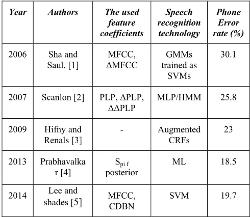
Much work has been in the field of phone recognition due to its wide applications. The summary of the most recent works on TIMIT database and the results are given in Table 1.

Table 1: Some of the works done on TIMIT and their results Phone

Error rate (%) Speech

recognition technology The used

feature coefficients Authors

Year

30.1 GMMs

trained as SVMs MFCC,

ΔMFCC Sha and

Saul. [1] 2006

25.8 MLP/HMM

PLP, ΔPLP, ΔΔPLP Scanlon [2]

2007

23 Augmented

CRFs -

Hifny and Renals [3] 2009

18.5 ML

Spi f posterior Prabhavalka

r [4] 2013

19.7 SVM

MFCC, CDBN Lee and

shades [5]

(2)

ISSN 2348 – 7968

529

3. Database and the Necessary Theories

3.1. TIMIT Database

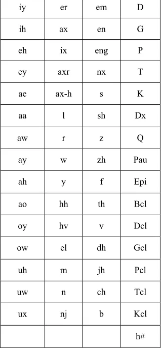
The continuous Corpus of TIMIT [6] acoustic-phonetic speech is made of English speech which is recorded using a microphone at a rate of 16 kHz and 16 bit resolution. This database includes 6300 sentences (5.4 hours) communicated by 630 speakers from 8 regional dialects of the United States. Each speaker articulated 10 sentences and all sentences are manually labeled based on the phone level. The main version of TIMIT is based on 61 phonetics shown in Table 2.

Table 2: 61 phones of TIMIT original phones

D em

er iy

G en

ax ih

P eng

ix eh

T nx

axr ey

K s

ax-h ae

Dx sh

l aa

Q z

r aw

Pau zh

w ay

Epi f

y ah

Bcl th

hh ao

Dcl v

hv oy

Gcl dh

el ow

Pcl jh

m uh

Tcl ch

n uw

Kcl b

nj ux

h#

One of the main reasons that this speech frame has become a standard for the of speech recognition community is that each sentence is labeled manually based on the phonetic level, and specified by allocation of the codes for the speakers’ number, gender and regional accent.

3.2. Pattern Recognition

There are different approaches to speech recognition. One of the most successful approaches is the recognition-based approach that almost all recent successful systems operate based on it. In this approach the speech is modeled based on some phonetic string (for example, word, syllable, three-phoneme or phoneme) and for the recognition the text of the speech is estimated by identifying these units and juxtaposing them together. Speech recognition systems, which use this approach, have two phases of training and testing. In the training phase, the patterns of each class which are the very phonetic units are modeled using some methods. The comparison of the input speech with the trained patterns is performed in the test phase in order to recognize the phonetic units in the speech. A speech recognition system consists of two main components of feature extraction and modeling unit (training phase), and the use of models or search (for test phase and use). In this structure, each of the related units can be performed in several ways.

3.2.1. Feature Extraction

(3)

ISSN 2348 – 7968

530 article the MFCC method explained in the next section is

used.

3.3. MFCC

The estimation of MFCC is based on human auditory system for an audio signal [7]. One of the reasons of the high performance of the coefficients is the high resolution. That is to say, small changes which are the results of this scale show their high effectiveness. Another strength point of this method is that besides eliminating the spectral structure, and summarizing the data, it reduces the correlation between the properties and improves the classification. The methodology for calculating the coefficients is explained below.

3.3.1. MFCC Calculation

Each frame of the audio signal is multiplied by a Hamming window and then the Discrete Fourier transform is taken from the resulting signal. The size of the Fourier transform has been calculated and the following steps are performed on the obtained envelope spectrum:

A: The signal spectrum is passed through 40 filters with Mel-scale bandwidth. These filters simulate the human auditory perception frequency separation. The primary13 filters with center frequency changes are linear (The frequency distance between the centers is 133/33 kHz) and the next 27 filters are logarithmic with center frequency changes ( the central frequency of the filter is 1.0711703 greater than the central frequency of the previous filter). Filters are triangular and each filter starts from the central frequency of the previous filter and ends in the center of the next central frequency and its maximum is within its own central frequency.

B: The logarithm of output filters is obtained.

C: In order to reduce the numbers of components of the feature vector the logarithmic values of the 40 output filters are multiplied by the discrete cosine transform and the obtained output equals the number of MFCC coefficients. Eq. (1) shows discrete cosine transform on the filters’ output:

)

2

1 (

cos(

]

[

]

[

1

0











M

m

M

m

n

m

S

n

C



(1)

Where

S

[

m

]

logarithm is the

m

_

th

output of filter,

M

is the total number of filters and

C

[

n

]

is equal to the

th

n

_

MFCC.

3.3.2. Delta Cepstral Coefficients

Cepstral coefficients express the features of speech signal and have a great benefit to enhance the accuracy of speech recognition. In order to maximize the accuracy of the system it is possible to use the derivations of these coefficients based on time. In fact the Cepstral coefficients model the static information of speech signal and they are sensitive to the status of dialects and their changes while the derivatives of the Cepstral coefficients contain dynamic information transfer data between different states of dialects. The integration of Cepstral coefficients and their derivatives can present better feature of the speech signal. The Cepstral coefficients derivation or the Delta Cepstral can be obtained from the Eq. (2):



 







2

.

4

1

j

j t i t

i

j

C

(2)

Where t i

C

is the

i

_

th

MFCC coefficient extracted from the

t

_

th

frame of each phone. To calculate the second derivatives of the coefficients or the Dlta- Delta Cepstral coefficients, the value of the Cepstral coefficient must be placed in equation 2.

3.4. Lifter

The purpose of extraction of signal feature coefficients is to use them in special analysis or application such as recognition. Hence all the measures and solutions will be applied in order to improve the recognition system. Classified liftering is one of the ways of improving the operations [8]. In this method, in an application such as speech recognition, when Cepstral coefficients (MFCC or LPCC) are used generally the lower coefficients are sensitive to slope of the range and the higher coefficients are sensitive to noise(the noise can be caused by such things as the calculation error or pluralization). In order to reduce the mentioned sensitivities the Cepstral vector is multiplied by a weight vector according to equation (3).

)

(

).

(

)

(

ˆ

_n

_C

_n

_W

_n

C



(3)

(4)

ISSN 2348 – 7968

531 linear, exponential and sinusoidal and the sinusoidal type

is used in this article and the related relation is as follows:

)

sin(

2

1 L

i

L

Wi







,

i



1 ,

2 ,...,

L

(4)

Where

L

represents the Cepstral features coefficients which equals 13.

3.5. Support Vector Machine

Support vector machine is a binary classifier. One of the advantages of this machine is the separation of the classes according to their distribution. This technique is an optimal separator that has shown its efficiency at classifying data in different applications [9].

3.5.1. Linear SVM

This type of classifier separates two classes with a border line. In the training phase, using all the training vectors and an optimization algorithm, a number of training samples separating the boundaries of the classes are obtained and these training samples are called the support vectors. In order to analyze the support vector machine it is assumed that the data are formed of two separate classes and the number of training vectors

x

_i is

L

. And the two classes are labeled

y

i



1

and

y

i





1

. In general, the separation boundary line is achieved by equation (5):

0 



b

wx

(5)

Where

x

is a point on the separating line and

w

is a perpendicular vector the separation boundary. Thus if

x

_i

is not a support vector,

y

_i

.(

w

.

x

_i



b

)



1

. The boundary line of the two separate classes is presented in Fig1.

Fig 1: the boundary line separating the two classes [10]

Given the choice of the values of b and w, there are many dividing lines that separate the two classes with zero error. To obtain the optimal separation boundary, the nearest training samples of two classes are obtained and then the distance from each other are calculated in a direction perpendicular to the boundaries that separate the classes. The Boundary separation between the two classes that has the maximum margin is the optimal separation and the Eq (6) is obtained.

1 )

.

(

w

x



b



y

_i _i ,

L

i



1 ,

2 ,...,

2

.

2

1 min

w

b w

(6)

To solve the optimization problem the indefinite Lagrange coefficient can be used. In this method the optimization problem reaches the Eq (7) in which the



_i is the Lagrange coefficient.





  





L

i L

j

L

i i j

j j i i

i

y

x

y

L ₁ ₁ ₁

,...,

2 (

.

)

]

1 [

max

1



 

L

i



1 ,...,



i



0

(7)





L

i i i

y

1

0 

By solving the above equation the value of

w

equals





L i

i i

i

y

x

w

1



and



_i is greater than zero for support

vectors and zero for non-support vectors. Then after finding w using Eq (8) for each support vector the

b

value is calculated and the final

b

will be obtained by averaging the total

b

.

0 ]

1 )

.

(

[

y

i

w

x

i



b





i



,

i



1 ,...,

L

(8) The final separation is obtained by Eq (9).

)

.

sgn(

)

(

x



w

x



b

(9)

3.5.2. Nonlinear SVM

(5)

ISSN 2348 – 7968

532 the new space using the previous equations and

replacement of

x

_i with



(

x

i

)

and considering an error

value for each vector the optimal separation boundary is calculated.

Optimization problem to find the optimal separation boundary reaches Eq (10)







 







L

i j j

j j L

i L

j

i i

i

y

x

y

L

i,..., ₁ ₁ ₁

))

(

).

(

2

1 [

max



 

L

i



1 ,...,

c





i



0

(10)





L

i i i

y

1

0 

In the above equation

c

is a constant value that specifies the error value the greater the value the greater the value of the error will be. In the above relation instead of using



a core function according to Eq (11) is used.

)

(

)

(

)

,

(

x

_i

x

_j

x

_i

x

_j

k





(11) So instead of the core function is placed and the optimization problem can be solved. Core functions are symmetric positive and definite. There are three important function that can be used including: A) polynomial function:

d

y

x

y

x

k

(

,

)



(

.



1 )

where

d

is the degree of the polynomial. B) GRBF1_:

)

2 exp(

)

,

(

₂

2



y

x

y

x

k





Where



is a Gaussian function width C) Sigmoid function:

)

.

(

tanh(

)

,

(

x

y



k

x

y





k

Where

k

and



are the Scale and intercept parameters In this paper of the type B (GRBF) is used.

3.6. Independent Component analysis

Independent component analysis is a signal processing technique for blind source separation, the feature extraction and signal detection. In this study we use the independent component analysis to eliminate the

1_{Generalized Radial Basis Functions}

dependence of the components of the feature vectors and as the name of this analysis suggests the main purpose of this conversion is to find a representation so that the components of the feature vectors are independent from each other. This is done by making all feature vectors covariance matrix entries zero except the main diagonal entries [11].

4. Practical Results

In this paper first the phonetics of the TIMIT database sampled at a rate of 16 KHz are extracted and then sequencing the similar phonetics 60 phonetic classes were obtained. The following steps are performed on the digital signal.

Pre emphasis: since the excited voiced phone of the larynx has -12

db

/

oct

slope and the radiation conversion function is in a way that the frequency response has increasing slope +6

db

/

oct

, in order to completely eliminate the effects of excitation and the effect of lips radiation the loading filter is performed by +6

oct

db

/

characteristic. This filter is known as Pre-emphasis. If

x

(

n

)

is the input speech signal, thus:

)

1 (

)

(

)

(

n



x

n



ax

n



y

,

0 .

9 

a



1

(15) Where

y

(

n

)

is the Pre-emphasized signal. In this paper

(6)

ISSN 2348 – 7968

533





N n

t

a

n

E

1

2

)

(

(16)







 





2

.

4

1

j

j t

t

j

E

(17)

Where the

E

_t is the frame energy of the

t

_

th

frame,

a

_t

is the sample of the

t

_

th

frame and

N

is the length of the frame. In this paper the length of each frame is equal to 320 samples (20 ms) and each frame has considered as 10 ms overlap with the previous frame. The last step before classification in order to equalize the value of the data and prevent the decrease system speed and accuracy of data) are normalized by Eq (18)

min max

min )

1 , 0 (

x

i i





(18)

In which

x

_max is the end and

x

_min is the beginning of the interval and

x

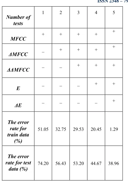
_i₍₀_,₁₎ is the normalized value in the interval (0, 1). Finally the classification is performed by training support vector machine based on the normalized feature vectors. The classification is summarized in Table 3. As the table 3 suggests adding the coefficients of the delta and MFCC delta and energy coefficient and energy- Delta improved the results significantly.

Table 3: Results of different feature vectors

Number of tests

1 2 3 4 5

MFCC + + + +

+

ΔMFCC _ + + +

+

ΔΔMFCC _ _ + + +

E _ _ _ + +

ΔE _ _ _ _ +

The error rate for train data

(%)

51.05 32.75 29.53 20.45 1.29

The error rate for test

data (%) 74.20 56.43 53.20 44.67 38.96

In addition to adding useful features to the feature vectors, one of the most useful applications of this work is to apply independent component analysis on the feature vectors. As shown in Fig 2, the results of each experiment in table 3 have significant error reduction after the independent component analysis compared with the results before it.

(7)

ISSN 2348 – 7968

534

5. Conclusion

In this paper, in order to classify the phonetics of English, speech signal of each sound is divided into 20 millisecond with 10 millisecond overlap. By using the appropriate feature vectors and ICA algorithm, a very good result with 4.93% error rate is obtained in classifying the test frames. These feature vectors contain 13 MFCC , 13 ∆MFCC, 13

∆∆MFCC coefficient 1 frame energy coefficient and 1 derived energy coefficient. Since the best result in other works contains 18.5% error the obtained results show significant improvement. The use of genetic algorithms to select the best features, in order to increase the classification accuracy is desired.

References

[1] F. Sha, and LK Saul, "Large margin Gaussian mixture modeling for Phonetic classification and recognition," in Acoustics, Speech and Signal Processing, 2006. Proceedings Icassp two thousand and six. 2006 IEEE International Conference on, 2 006, pp. II.

[2] P. Scanlon, DPW Ellis, and RB Reilly, "Using experts for improved speech recognition broad Phonetic group," Audio, Speech, and Language Processing, IEEE Transactions on, vol. 15, pp. 803-812, 2007 .

[3] Y. Hifny, and S. Renals, "Speech recognition using augmented Conditional random fields," Audio, Speech, and Language Processing, IEEE Transactions on, vol. 17, pp. 354-365, 2009.

[4] R. Prabhavalkar, TN Sainath, D. Nahamoo, B. Ramabhadran, and D. Kanevsky, "An evaluation of posterior modeling techniques for Phonetic recognition," in Acoustics, Speech and Signal Processing (Icassp), the 2,013th IEEE International Conference on , in 2013, pp . 7165-7169.

[5] H. Lee, P. Pham, Y. Largman, and A. Y. Ng, "Unsupervised learning feature for audio classification using Convolutional deep belief networks," in Advances in neural information processing systems , 2,009, pp. 1096-1104.

[6] J. S. Garofolo, L. F. Lamel, W. M. Fisher, J. G. Fiscus, and D. S. Pallett, "DARPA CD-ROM Timit acoustic-Phonetic Continous speech corpus. NIST speech disc 1 to 1.1," NASA STI / Recon Technical Report N, vol. 93, pp. 27403, 1993.

[7] S. Davis, and P. Mermelstein, "Comparison of parametric Representations for Monosyllabic word recognition in continuously spoken Sentences," Acoustics, Speech

and Signal Processing, IEEE Transactions on, vol. 28, pp. 357-366, 1980.

[8] K. K. Paliwal, " On the use of filter-bank energies as features for robust speech recognition," in Signal Processing and Its Applications, 1999. Isspa'99. Proceedings of the Fifth International Symposium on , the 1999th, pp. 641-644.

[9] C. Cortes and V. Vapnik, "Support-vector networks," Machine learning, vol. 20, pp. 273-297, 1995.

[10] D. Meyer and F. T. Wien, "Support vector machines," The Interface to Libsvm in package E1071, January, vol. 10, 2014 .