Article
1
Calculation of Maximum Total Supply Capacity of
2
Three-Phase Unbalance Distribution Network Based
3
on Mixed Integer Second-Order Cone
4
Jieyun Zheng 1, Shiyuan Ni 1, Pengjia Shi 1, Guilian Wu 1, Ri’an Wang 2,*, Chenying Yi 2 and
5
Zhijian Hu 2
6
1 State Grid Fujian Economic Research Institute, Fuzhou 350000, China;
7
2 School of Electrical Engineering and Automation, Wuhan University, Wuhan 430072, China;
8
[email protected] (J.Z.); [email protected] (S.N.); [email protected] (P.S.); [email protected]
9
(G.W.)
10
* Correspondence: [email protected]
11
Abstract: Considering the fault "N-1" checksum and the power flow, the single-phase power flow
12
model is further transformed into a three-phase power flow model, and the asymmetry of the
13
three-phase power flow is measured by the three-phase unbalance factor. The calculation model is
14
linearized by the second-order cone relaxation and the Big-M method. At the same time, the load
15
response and distribution network reconstruction are used to improve the reliability of the power
16
supply network to cope with the power failure. The relationship between power supply capability
17
and power flow constraints, main transformer capacity and distributed power parameters is
18
analyzed by IEEE 33-node three-phase power distribution system. The feasibility of the proposed
19
model and the accuracy of the second-order cone relaxation are verified by numerical examples,
20
which provides a technical reference for distribution network planning.
21
Keywords: distribution network; total supply capacity; second-order cone relaxation; power flow
22
calculation; load response; Big-M method; three-phase unbalance degree
23
24
1. Introduction
25
The total supply capacity (TSC) of distribution network refers to the maximum load supply
26
capacity within a certain power supply range based on interconnections of main transformers when
27
meeting the “N-1” guideline and actual operation constraints [1]. TSC characterizes the power
28
supply reliability of distribution network, and the accurate calculation of it is conducive to the
29
planning and refined load management of distribution network in line with the increasing load
30
demand.
31
At present, the research on the calculation of power supply capacity has experienced three
32
stages in its development process [2-3]. In the first stage, the power supply capacity was evaluated
33
based on the substation capacity and capacity-load ratio. However, the effect of the subordinate
34
network on the power supply capacity had not been considered at this stage, and the calculation
35
results cannot reflect the power supply requirements precisely. The second stage is the initial stage
36
that considered the substation capacity and the power transfer capability of network at the same
37
time, but only the feeder load was taken into account in the evaluation of power transfer capability,
38
which may lead to deviation. And the third stage is the precise theoretical modeling stage of power
39
supply capacity [4], taking into account the “N-1” guideline, substation capacity and power transfer
40
capability of network. Reference [5] proposed a calculation method of power supply capacity based
41
on interconnections of main transformers and “N-1” guideline. Considering the two points that
42
mentioned above, the calculation method of power supply capacity considering the contact capacity
43
and the short-time overload problem of the main transformers was proposed in reference [6], which
44
can help to improve the accuracy of calculation results. Based on power flow calculation, reference [7]
45
established an TSC model considering the voltage drop and network loss, which considers the
46
interconnections between feeders and the “N-1” fault of main transformers and feeders at the same
47
time. The model and the calculation method can be applied to the field of the operation in
48
distribution network.
49
In recent years, with the development of smart grid and power distribution automation, the
50
proportion of some equipment that access to distribution network has been increasing, such as
51
distributed generation (DG) and flexible load, which has certain impact on the planning and
52
operation of distribution network. This phenomenon should be considered in the calculation of
53
power supply capacity, and some studies have considered the impact of the above factors in the
54
calculation process. Taking the maximum expected value of the load amplification factor under the
55
typical DG output scenario as the optimization goal, reference [8] established a calculation model of
56
TSC, which considers the site selection of DG and network reconfiguration. The calculation results
57
show that the access of DG is beneficial to the improvement of TSC. Reference [9] established a
58
two-layer optimization model for TSC considering the uncertainty of DG output. In this model, the
59
economic operation of the active distribution network is considered, but the “N-1” safety guideline
60
is not included in the constraints. In reference [10], the TSC model including users grading and
61
interaction between demand-side and grid was established. The load in demand-side response is
62
considered as interruptible load and emergency load, and simulation of the paper shows that the
63
interaction between users and grid can improve the TSC of distribution network. It can be seen from
64
the above research status that both DG and flexible load can play a role in improving TSC, but few
65
studies have considered the relationship between them in the calculation model of TSC.
66
One problem that should also be considered when calculate TSC is that after the equipment
67
such as DG and flexible load are connected to the distribution network in phase, the original
68
three-phase asymmetry of the distribution network will be more serious. If the single-phase
69
equivalent model in the previous study is continuously used in the analysis of the TSC, the
70
calculation results will be out of the actual situation of the distribution network and might also lead
71
to a large deviation [11-13]. Therefore, the three-phase asymmetry of the distribution network must
72
be fully considered.
73
In summary, based on the mixed integer second-order cone optimization method, the
74
following solutions are proposed by combining the three-phase power flow calculation model
75
proposed in [16]:
76
1. Fully consider the three-phase asymmetry of the distribution network, establish a mathematical
77
model of each asymmetry factor, and accurately calculate the TSC of the distribution network
78
through the three-phase power flow calculation method and the simulation of “N-1” fault.
79
2. Use the distribution network reconfiguration model to enhance the flexibility of TSC, and
80
transform the nonlinear model established by the Big-M method into a mixed integer model
81
according to the method of [20]. At the same time, based on the actual situation, set the
82
minimum load demand for all load nodes and add part of the unimportant load into the
83
regulation range of load response.
84
Through the simulation of the improved IEEE 33-node three-phase distribution system, the
85
effectiveness of the proposed model and scheme was confirmed.
86
2. Three-Phase Power Flow Model
87
According to Kirchhoff's law, the sum of the power that flowing into the node is equal to the
88
sum of outflows in distribution network. Therefore, for any node j, the three-phase active and
89
reactive power can be described as:
90
= + +
= + +
,DG ,T
,DG ,T
j j j j
j j j j
P P P P
Q Q Q Q (1)
91
•
A, B, C
refers to phase A, B and C;• j
P and Qj refer to the three-phase active power and reactive power of the load demand at
93
node j, respectively;
94
•
jP and
Qj refer to the net injection quantities of three-phase active and reactive power,95
respectively;
96
• ,DG
j
P and Qj,DG refer to the three-phase active power and reactive power of the DG at node j,
97
respectively;
98
• ,T
j
P and Qj,T refer to the three-phase active and reactive power input by the substation to
99
node j, respectively.
100
For the radial distribution network, the power flow formulas in the form of distflow [14] can be
101
described as shown in formula (2).
102
(
)
(
)
− + =
− + =
= − + + +
2
( ) ( )
2
( ) ( )
2 2 2 2 2
( )
( )
( ) ( ) 2( ) (( ) ( ) ) ( )
ij ij ij j jk
i u j k v j
ij ij ij j jk
i u j k v j
j i ij ij ij ij ij ij ij
P I r P P
Q I x Q Q
V V r P x Q r x I
(2)
103
• u j( ) refers to the set of the head nodes of branches with j as the end node in the distribution
104
system;
105
• v j( ) refers to the set of the end nodes of branches with j as the head node;
106
• ij
P and Qij refer to the three-phase active and reactive power flowing on branch ij ,
107
respectively;
108
• ij
r and xij refer to the three-phase resistance and reactance of branch ij, respectively;
109
• jk
P and Qjk refer to the three-phase active and reactive power flowing on branch jk,
110
respectively;
111
•
i
V and Vj refer to the three-phase voltage amplitudes of node i and node j, respectively;
112
The second-order cone relaxation Iij is the current amplitude of branch ij, which can be
113
calculated by formula (3).
114
+ =
2 2
2
2 ( ) ( ) ( )
( )
ij ij
ij
i
P Q
I
V (3)
115
There are some non-convex terms such as quadratic terms and negative quadratic terms in the
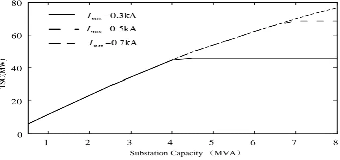
116
power flow formulas that mentioned above, which will make the optimization problem with power
117
flow constraints difficult to solve. The solution methods of this problem mainly include seeking local
118
optimal solutions, approximate linearization and convex relaxation for power flow constraints
119
[14-15]. Among those methods, the convex relaxation technique is widely applied to ensure the
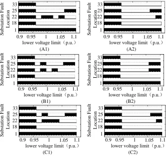
120
efficiency of the algorithm and the optimality of the solution. Therefore, for the above-mentioned
121
power flow formulas, the second-order cone programming (SOCP) method has good applicability
122
[16]. Replace the variables in formula (2) and formula (3) as follows:
123
=
+
= =
2 2,
2 2
2 2,
2, ( )
( ) ( ) ( )
j j
ij ij
ij ij
i
v V
P Q
i I
v
(4)
124
The second term in formula (4) can be further relaxed and converted into a standard
125
second-order cone type:
126
− T + 2, 2, 2 2, 2,
[2Pij 2Qij i ij v i] i ij v i (5)
127
The final SOCP form of the power flow formulas can be described as:
(
)
(
)
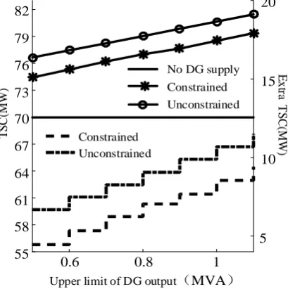
− + =
− + =
= − + + +
− +
2,
( ) ( )
2,
( ) ( )
2 2
2, 2, 2,
T
2, 2, 2 2, 2,
2( ) (( ) ( ) )
[2 2 ]
ij ij ij j jk
i u j k v j
ij ij ij j jk
i u j k v j
j i ij ij ij ij ij ij ij
ij ij ij i ij i
P i r P P
Q i x Q Q
v v r P x Q r x i
P Q i v i v
(6)
129
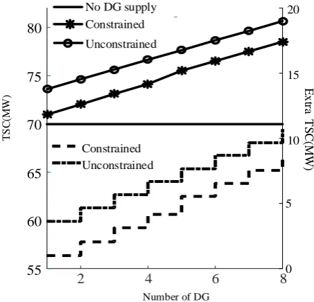
3. Factors Affecting Three-Phase Asymmetry of Distribution Network
130
Distribution network contains a large number of asymmetric lines and loads, which makes it
131
possess the characteristic of three-phase asymmetric. After the flexible load and the DG that operate
132
in a non-full-phase state connected to the distribution network, the asymmetry characteristic
133
appears to be more significant. In the above situation, if the traditional single-phase equivalent
134
model is still used in the analysis, a large error will result. Therefore, in order to comprehensively
135
evaluate the power demand of users and accurately calculate the TSC of distribution network, it is
136
necessary to analyze the typical factors of three-phase asymmetry and introduce the concept of
137
three-phase unbalance factor to describe the unbalance degree of distribution network.
138
3.1. Three-phase Asymmetric Load
139
The asymmetry of three-phase load is the main cause of three-phase unbalance in power system.
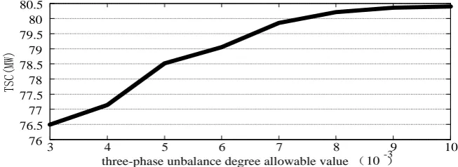
140
The asymmetry of load mainly comes from the uneven distribution of single-phase load of power
141
users in the system [17]. When calculating the TSC of distribution network, the equivalent of a
142
three-phase load to a single-phase model will not accurately assess the actual demand of each phase
143
load, so the load conditions of each phase should be considered separately.
144
3.2. Three-phase Asymmetric DG
145
When a single-phase DG (such as single-phase photovoltaic generator, single-phase wind
146
turbine, etc.) is connected in distribution network, the output of each phase is usually not completely
147
equal due to the uncontrollable factors such as geography and climate, which will make the
148
distribution network that is originally not a fully one more asymmetrical [18]. When analyzing a
149
distribution network containing DG, the influence of DG on the three-phase unbalance should be
150
fully considered. This paper refers to [16] to equivalently treat the DG into PQ types.
151
3.3. Three-Phase Unbalance Factor of Node Voltage
152
The degree of three-phase asymmetry of distribution network is described by the voltage
153
unbalance factor, which can be described as follows [19]:
154
= −
avg
avg
i i
i
i
V V
V (7)
155
•
i
V refers to the voltage amplitude of phase ;
156
• avg
i
V refers to the average value of the three-phase voltage amplitude.
157
In Section 2, the node voltage amplitude can be replaced according to formula (4), and the
158
following formula can be obtained:
159
−
=
=
avg 2 , 2 , 2 , avg
2 ,
2 , avg
2 , 3
i i
i
i
i i
v v
v
v v
(8)
160
Define as the maximum value of voltage unbalance factor. When the condition 2,i is
161
satisfied, the condition i must also be satisfied. The specific derivation process is shown in the
Appendix. Therefore, the variables in the voltage unbalance factor can be replaced by the relaxed
163
variables in the SOCP-type power flow formulas, as shown in the first term of formula (8).
164
4. Calculation Model of TSC
165
4.1. Objective Function
166
The objective is given by
167
B i i
Max P (9)
168
+
, ( )2,
( )
B
t n
i ij ij
i n ij
Max P I r (10)
169
•
i
P refers to the active load demand;
170
• B refers to the set of all nodes;
171
• refers to the weight of the loss factor in the objective function.
172
The meanings of the formulas are as follows:
173
• Equation (9) refers to the maximum active load supplied by the entire distribution network.
174
• In order to consider the influence of network loss on the power supply capacity and minimize it,
175
the formula (9) is converted into the formula (10).
176
The “N-1” guideline means that when any power supply component fails alone, the system
177
continues to supply power to the original load. It should be noted that the line fault has less impact
178
on the TSC than the substation fault. Therefore, only the substation to perform “N-1” needs to be
179
verified.
180
4.2. Constraints
181
, (n)= , (n) 2
2 , ( )
t t
ij ij
I I (11)
182
(
)
− + =
, (n) , (n)
, (n)
, (n) 2 ,( ) ( )
t t t t
ij ij ij j jk
i u j k v j
P I r P P (12)
183
= + +
, (n) , (n) , (n), ,T
t t t
j j j DG j
P P P P (13)
184
(
)
− + =
, (n) , (n)
, (n)
, (n) 2,( ) ( )
t t t t
ij ij ij j jk
i u j k v j
Q I x Q Q (14)
185
= + +
, (n) , (n) , (n), ,T
t t t
j j j DG j
Q Q Q Q (15)
186
• , (n) 2 ,
t ij
I refers to the current squared term of line ij. Use this auxiliary variable instead of the
187
quadratic term to eliminate the nonlinear variables;
188
• n n( =1, 2, 3,L Ntrans) refers to the serial number of the substation, and Ntrans refers to the total
189
number of substations;
190
• t(n) refers to the node number corresponding to the substation n;
191
• , (n) ,
t j DG
P and , (n) ,
t j DG
Q refer to the active and reactive input power of DG at node j, respectively;
192
• , (n) ,T
t j
P and
, (n)t jQ refer to the active and reactive input power of the substation at node j,
193
respectively.
194
Equations (12) - (15) are the balance constraints of active and reactive power at nodes in power
195
flow constraints. The balance formula of the power at node consists of three parts: the first part is the
196
power flow of line ij, the second part is the power flow of line jk, and the last part is the node
197
input power flow. It should be noted that in the case of failures of each substation, the load of the
198
node is constant.
199
0, 0
j j
P Q (16)
200
, (n) , (n)
, 0, , 0
t t
j DG j DG
P Q (17)
, (n) , (n)
,T 0, ,T 0
t t
j j
P Q (18)
202
Equations (16) - (18) represents the flow direction of power. The symbol is positive when the
203
power flows to, and it is negative when the power flows out the node.
204
, (n) = , (n) 2
2 , ( )
t t
j j
V V (19)
205
, (n) = , (n)− , (n)+ , (n) + 2+ 2 , (n)
2 , 2 , 2( ) (( ) ( ) ) 2 ,
t t t t t
j i ij ij ij ij ij ij ij
V V r P x Q r x I (20)
206
+
=
2 , (n) 2 , (n) 2 , (n)
2, , (n)
2, ( t ) ( t )
ij ij
t
ij t
i
P Q
I
V (21)
207
, (n) , (n) , (n)− , (n) T , (n)+ , (n)
2, 2, 2 2, 2,
[2Pij t 2Qijt I ijt V it ] I ijt V it (22)
208
• , (n) 2,
t j
V replaces the quadratic term of , (n)t j
V .
209
According to the power flow constraints for branch in the form of distflow, the branch should
210
satisfy equations (20) - (21). According to the form of the second-order cone, the formula (21) can be
211
deformed into the formula (22).
212
, (n)tT =
i base
V V (23)
213
,min 2 , (n) ,max 2 2,
( ) t ( )
i i i
V V V (24)
214
, (n) ,max 2 2 ,
0 t ( )
ij ij
I I (25)
215
, (n)+ , (n) , T , T
t t
j j T
P Q S (26)
216
• ,max
i
V and Vi,min refer to the maximum voltage limit and minimum voltage limit of node i,
217
respectively;
218
• ,max
ij
I refers to the maximum allowable current of branch ij;
219
• ST refers to the maximum capacity of the substation;
220
• Vbase refers to the reference voltage of the distribution network.
221
In the formulas that mentioned above, formula (24) indicates the range of voltage values for all
222
nodes; formula (25) indicates the range of current values for all branches; formula (26) indicates the
223
capacity of the substation.
224
, ( )= =
, 0, ( )
t n i T
P i t n (27)
225
, ( )= =
, 0, ( )
t n i T
Q i t n (28)
226
Equation (27) and equation (28) indicate that when a substation fails, the substation of the
227
corresponding node has no input power.
228
, (n)
2,
0 t , 0,1 ,
ij ij ij S
I S M S j (29)
229
− − + − , (n)+ , (n) + 2+ 2 , (n)
2, (1 ) 2, 2( ) (( ) ( ) ) 2,
t t t
j ij i ij ij ij ij ij ij ij
V M S V r P x Q r x I (30)
230
− + − , (n)+ , (n) + 2+ 2 , (n)
2, (1 ) 2, 2( ) (( ) ( ) ) 2,
t t t
j ij i ij ij ij ij ij ij ij
V M S V r P x Q r x I (31)
231
• ij
S refers to the state of the circuit breaker on the line. When =0 ij
S , it indicates that the circuit
232
breaker is open, and when =1 ij
S , the circuit breaker is in the connected state.
233
• M refers to a large enough value.
234
Equation (29) is processed by Big-M method, which can transform nonlinear problems into
235
mixed integer linear programming. When the circuit breaker is disconnected, equation (20) is no
236
longer applicable. Equations (30) and (31) transform the equation relationship into two inequality
237
relations. When =1 ij
S , the two inequalities are equivalent to the original constraint (20); when
238
=
0 ij
S , as long as M is sufficiently large, there is no limit between the voltages across the line.
239
0,1 ,
= ,maxi B i B N (32)
,min , ( ) ,max
, , ,
i B B B
t n
i DG i DG i i DG
P P P (33)
241
,min , ( ) ,max
, , ,
i B B B
t n
i DG i DG i i DG
Q Q Q (34)
242
•
i B refers to the investment decision variable of DG. When
=1
i B , it indicates that DG is
243
access to the node.
244
• N,max refers to the total number of DG invested.
245
The input power of the DG is also processed by Big-M, as shown in equations (33) and (34).
246
, (n)= A, (n)− avg, (n) 2,i 2,it
A t t
i V V (35)
247
, ( )= , ( )− , ( )2, 2,
avg t n B t n B t n
i V i V i (36)
248
, ( )= , ( )− , ( )2, 2,
avg t n C t n C t n
i V i V i (37)
249
+ +
=
, (n) , (n) , (n)
2, 2 2
avg, (n) 2,
3
A t B t C t
i ,i ,i
t i
V V V
V (38)
250
, (n) , (n) , (n) max Max( A t , B t , C t )
i i i (39)
251
• A t, (n)
i ,
, (n)
B t
i and
, (n)
C t
i refer to the voltage unbalance factor of each phase of the node;
252
• avg, (n) 2,
t i
V refers to the upper limit of the unbalanced factor.
253
In the above formulas, equations (35) - (38) refer to the calculation process of three-phase
254
unbalance; formula (39) means that the imbalance of the voltages of the respective phases cannot
255
exceed the allowable upper limit.
256
− ,
j j j need
P P (40)
257
• j refers to the proportion of load demand reduction, and the value of it ranges from 0 to 1.
258
5. Simulation and Analysis
259
The simulation is programmed by the MATLAB platform and the Cplex solver in the Yalmip
260
platform is used for optimization. The development environment is MATLAB R2014a. The test
261
system's processor parameters are Intel(R) Core(TM) i5-4200H CPU clocked at 2.8GHz, memory is
262
4GB, and the operating system is Windows7 64bit.
263
Take the IEEE 33-node three-phase asymmetric power distribution system as example. The
264
specific line parameters and the minimum load demand of each load node are detailed in [22]. The
265
reference voltage of this system is 12.66 kV, and the lower limit of the node voltage is 0.9 p.u. The
266
maximum capacity of the substation is 7 MVA, the maximum allowable current of the feeder line is
267
0.7 kA, the upper and lower limits of the distributed output are 0.1 MVA and 1 MVA, respectively,
268
and the circuit breaker access positions are line 2-3 and line 4-5. The three-phase unbalance is
269
allowed to be 10-3.
270
In a traditional distribution network, a single power supply generally supplies power to all
271
loads. When a power supply fails, all load nodes will face a significant risk of power outage.
272
Therefore, the distribution network with high reliability requirements generally uses dual power
273
supply or multiple power supply for important loads. When a single substation fails or is
274
overhauled, the load facing the risk of power outage can be transferred to other substations to
275
improve the reliability of the system. Based on the above considerations and ease of research and
276
analysis, the IEEE 33-node system of the distribution network has been modified appropriately, and
277
nodes 1, 18, 22, 25 and 33 are set as substation access points, as shown in Figure 1.
1 2 3 4 5 6 7 8 9 10 19
11 12 13 14 15 16 17 18
20 21 22
23 24 25
26 27 28 30 31 32 33
DG
DG DG DG DG
DG
DG
DG T1
T3
T2
T4
T5
279
Figure 1. The IEEE 33-bus distribution network
280
5.1. The Influence of the Node Voltage Allowable Lower Limit and Substation Capacity on TSC
281
The relationship between TSC substation capacity and TSC is shown in Figure 2. Due to the
282
limitation of the maximum current Imax allowed by the line, when the substation capacity reaches a
283
certain value, it has no effect on the promotion of TSC. By observing the curves of three different
284
trends, it can be found that the maximum current allowed by different lines will change the upper
285
limit of the influence of the capacity of the substation. In a certain range of substation capacity, the
286
maximum allowable current change of the line has no effect on the TSC.
287
Substation Capacity (MVA)
TS
C
(MW
)
1 2 3 4 5 6 7 8
0 20 40 60 80
288
Figure 2. Impact of substation capacity on TSC
289
The relationship between the switching states of circuit breaker and the node voltage lower
290
limit values is shown in Figure 3.
291
In Figure 3, the ordinate indicates the node number corresponding to the faulty substation, and
292
the five substations correspond to five bar graphs. When the circuit breaker is closed, the
293
corresponding position in the bar graph is a rectangle. When the circuit breaker is disconnected, the
294
corresponding position in the bar graph is a straight line. Figure 3 is divided into six parts based on
295
the phase and breaker number. Figure 3 shows that all circuit breakers are closed when the lower
296
voltage limit is lower, because the lower voltage lower limit allows the nodal load to obtain the
297
power supply to the farther substation. For example, when line 4-5 is in the connected state, node 5 is
298
able to obtain the power supply to the substation at node 18 and node 33. This effect is more
299
pronounced as the substation capacity is smaller.
300
Conversely, when the lower voltage limit is higher, the substation has to select a load with a
301
closer distance. At the same time, once the circuit breaker is opened, the voltage relationship
302
between the two ends of the circuit breaker is no longer limited, which further alleviates the
303
hindrance of voltage constraints to the improvement of power supply capacity. Therefore, most of
the circuit breakers are in the open state. Taking node 5 as an example, the voltage loss is smaller
305
from node 5 to node 22 and node 25 compared to node 5 to node 18 and node 33, which makes the
306
closure of circuit breaker 1 more advantageous and TSC boost. Similarly, when the substation of
307
node 22 and node 25 fails, the circuit breaker is also in a closed state when the minimum allowable
308
voltage value is large. In summary, when the distribution network responds to changes in the
309
allowable value of the lower voltage limit, the presence of the circuit breaker makes the TSC upgrade
310
more flexible.
311
18 22 25
1 33 18 22 25
1 33
18 22 25
1 33
18 22 25
1 33
18 22 25
1 33
18 22 25
1 33
0.9 0.95 1 1.05 1.1
lower voltage limit(p.u.)
(A1)
0.9 0.95 1 1.05 1.1
lower voltage limit(p.u.)
(A2)
0.9 0.95 1 1.05 1.1
lower voltage limit(p.u.)
(B1)
0.9 0.95 1 1.05 1.1
lower voltage limit(p.u.)
(B2)
0.9 0.95 1 1.05 1.1
lower voltage limit(p.u.) (C1)
0.9 0.95 1 1.05 1.1
lower voltage limit(p.u.) (C2)
S
ubs
ta
ti
on
F
aul
t
L
oc
at
ion
S
ubs
ta
ti
on
F
aul
t
L
oc
at
ion
S
ubs
ta
ti
on
F
aul
t
L
oc
at
ion
S
ubs
ta
ti
on
F
a
ul
t
L
oc
at
ion
S
ubs
ta
ti
on
F
aul
t
L
oc
at
ion
S
ubs
ta
ti
on
F
a
ul
t
L
oc
at
ion
312
Figure 3. Relationship between voltage lower limit and circuit breaker status
313
Figure 4 shows the optimization results of the TSC under the constraints of the substation
314
capacity and lower voltage limit. Figure 4 shows that the TSC analysis can provide guidance for the
315
planning and design of substation capacity in the distribution system based on the corresponding
316
voltage constraints in order to make more efficient use of the capacity of the transformer. Figure 4(b)
317
and Figure 4(c) show that as the lower voltage limit increases, the TSC gradually decreases. When
318
the voltage lower limit is below the critical value, the TSC is substantially unaffected.
319
It should be additionally noted that the higher the voltage lower limit represents the higher the
320
requirement for voltage quality, but it does not mean that the voltage level must be used as a
321
decision variable in the actual planning. In actual situations, it can be decided according to different
322
design requirements.
3 4 5 6 7 8 0.8 0.85 0.9 0.95 1 1.05 1.1 1.15
0.8 0.9
1 1.1
1.2 2
4
6
8 20
40 60 80
30 40 50 60 70
30 40 50 60 70
TSC
(MW
)
TSC
(MW
)
TSC
(MW
)
(a)
(b) (c)
Substation Capacity (MVA) lower voltage limit(p.u.)
lower voltage limit(p.u.) Substation Capacity(MVA)
324
Figure 4. Synergy relationship between TSC and substation capacity and voltage lower limit
325
5.2. TSC Analysis Taking into Account Single-Phase DG Access
326
The case of single-phase DG access is considered to highlight the effects of three-phase
327
asymmetry. The relationship between the upper limit of DG output and TSC is shown in Figure 5.
328
0.6 0.8 1
55 58 61 64 67 70 73 76 79 82
5 10 15 20
No DG supply
Constrained
Upper limit of DG output(MVA)
T
S
C
(MW
)
E
x
tra
T
S
C
(MW
)
Unconstrained
Constrained Unconstrained
329
Figure 5. The impact of the upper limit of DG output on TSC
330
Figure 5 is a double ordinate form that can be divided into two parts. The first part is to evaluate
331
the TSC after a single-phase distributed power access system. The second part shows the TSC
332
benefits of DG, which is shown in the lower part of the figure. Both parts give a comparison of the
333
presence or absence of three-phase unbalance constraints. In order to highlight the asymmetry of the
334
distributed power supply, only the distributed power supply of phase A is considered. Figure 5
335
shows that after accessing the distributed power supply, the TSC has a significant increase and
336
brings a power supply capability that exceeds the sum of the maximum output of the distributed
337
power supply. This is because the distributed power supply can take advantage of short-distance
338
transmission and make up for the power loss caused by the failure of each substation. It can directly
339
transmit power to users facing the risk of power outage without receiving power from other
340
substations remotely. However, with the increase of the upper limit of DG output, the benefits
brought by DG are no longer obvious, and the growth trend of TSC is basically the same as the
342
increase of the maximum output of DG. This shows that the extra distributed power output will no
343
longer supply power to remote loads, but only increase the power supply potential of the DG access
344
node.
345
A detailed observation of Fig. 5 reveals that after the addition of the three-phase unbalance
346
constraint, TSC is limited by the asymmetric variation of the three-phase current distribution caused
347
by the access of the single-phase distributed power source. With the upper limit of DG output, the
348
growth trend of TSC considering the three-phase unbalance constraint is roughly the same as that
349
without considering the constraint. This is because the remaining distributed power output is
350
limited by the imbalance constraints, making it impossible to supply load of remote nodes through
351
the line transmission. Eventually, only the load on the access node can be selected for supply.
352
Assuming that there are only eight alternative DG access nodes, the simulation results shown in
353
Figure 6 are obtained by controlling the number of access points of the distributed power supply,
354
wherein the maximum output of each distributed power supply is 1 MVA.
355
2 4 6 8
55 60 65 70 75 80
0 5 10 15 20
T
S
C
(MW
)
Number of DG
No DG supply Constrained Unconstrained
Constrained Unconstrained
E
x
tr
a
T
S
C
(MW
)
356
Figure 6. The impact of the upper limit of DG on TSC
357
The relationship between the upper limit of the number of DGs and the average output of DG is
358
shown in Fig. 7. The ordinate of Figure 7 represents the average power supply benefit from each
359
distributed power source. This benefit is obtained by the relationship between the extra TSC and the
360
number of DGs.
361
1 2 3 4 5 6 7 8
0 1 2 3 4
Constrained Unconstrained
Number of DG
Ave
ra
ge
bene
fit
f
rom
DG
(
M
V
A
)
362
Figure 7. The relationship between the upper limit of DG quantity and the average output of DG
363
Figures 6 and 7 show that, in particular, when the three-phase unbalance constraint is not taken
364
into account, the distributed power source brings the power supply capability to a quantity that
365
exceeds its own maximum output sum. The power supply capacity gain of the station is also
366
gradually reduced as the number of DG units increases. In the power grid structure, the distributed
power flow distribution of some distributed power sources overlaps, so that in the case of partial
368
faults, these distributed power supplies maintain lower power output in order to avoid line power
369
crossing. In addition, after accounting for the three-phase unbalance constraint, the average power
370
supply capability gain from the distributed power supply is roughly equal to the upper limit of the
371
distributed power output. Since the optimization trend of the model is to obtain more power supply
372
capability, the DG output that cannot flow have to be absorbed locally.
373
The relationship between three-phase unbalance and TSC is shown in Figure 8. Figure 8 shows
374
that as the allowable value of the three-phase unbalance is increased, the TSC gradually rises and the
375
rising trend is slower. Combined with the analysis of Figure 6 and Figure 7, it can be seen that
376
because the DG is limited by the three-phase unbalance degree, it can more flexibly compensate for
377
the power failure loss caused by the distribution network failure.
378
76 76.5 77 77.5 78 78.5 79 79.5 80 80.5
3 4 5 6 7 8 9 10
TSC
(MW
)
three-phase unbalance degree allowable value ( 10 -3)
379
Figure 8. TSC and three-phase unbalance degree allowable value relationship diagram
380
5.3. TSC Analysis Taking Into Account Load Response
381
For the sake of analysis, only the distribution network of phase A is studied. The distribution of
382
load output at each point of phase A is shown in Figure 9.
383
The histogram in Fig. 9 shows the load distribution of each node, the white column indicates the
384
load distribution after considering the load response, and the black portion indicates the load
385
distribution without considering the load response, where nodes 7, 8, 29, 30 and 31 are controllable
386
load node. When the load demand of the controllable load nodes is reduced, the power supply of
387
some nodes is greatly improved, and the overall power supply capacity in phase A is increased from
388
21.8 MVA to 22.1 MVA. This shows that the power distribution system can improve the power
389
supply capability of some nodes and the overall network through load shedding under the premise
390
of meeting security constraints.
391
0
10
20
30
40
0
2
4
6
Response
No Response
Node number
M
axi
m
um
s
upp
ly
loa
d
of
the
node
(
MW
)
392
Figure 9. Distribution of load output of each node in phase A
393
5.4. The Influence of the Proportional Coefficient on TSC and the Verification of the Accuracy of the SOCP
394
Figure 10 shows that as the coefficient increases, the TSC and system network losses decrease.
395
The simulation results show a higher level of network loss compared to the method of [21]. This is
396
because the load distribution in the literature [21] is mostly at the front end of the network and does
397
not require long-distance transmission of power. However, in order to meet the load requirements of
398
each node in this paper, the supply of power has to be transmitted by long-distance lines, which
results in an undesired network loss. Figure 10 provides guidance recommendations that help to
400
trade off between choosing a larger TSC and a smaller network loss.
401
10 10 1 3 5 10 20 40
0 20 40 60 80
Network loss TSC
-2 -1
Net loss coefficient
T
SC
/N
et
w
or
k
lo
ss
(
MW
)
402
Figure 10. Network loss coefficient and relationship between TSC and network loss
403
5.5. TSC Result Compared with Other Method
404
The infinite norm of the second-order cone relaxation error vector defining the branch is as
405
follows [16]:
406
+
= −
2 2
2
2 ( ) ( ) Gap ( )
( )
ij ij
ij
i
P Q
I
V (41)
407
Figure 11 shows that as the network loss coefficient increases, the line average current and
408
second-order cone error of the system gradually decrease. This shows that by controlling the
409
objective function, the error of the second-order cone relaxation can be effectively adjusted.
410
10 10 1 3 5 10 20 40
0 0.1 0.2 0.3
0 0.002 0.004 0.006 0.008 0.01
Average current
Error
-2 -1
Net loss coefficient
A
ve
ra
ge
c
ur
re
nt
(
kA
)
E
rro
r
(
kA
)
411
Figure 11. Network loss coefficient and average current and error relationship
412
Establish a network model as shown in Figure 12 according to the method in [2]. The TSC
413
obtained by this method is 105 MVA, and the result is significantly larger than the calculated result
414
when the power flow distribution is taken, and exceeds the sum of the capacities of all the
415
transformers. This result indicates that the node voltage, branch current, and three-phase unbalance
416
constraints all have critical limitations on TSC.
417
T1
T2
T3
T5
T4
418
Figure 12. Schematic diagram
5. Conclusions
420
1. Compared with previous studies, this paper incorporates the three-phase power flow model
421
into the calculation of maximum power supply capacity. The three-phase power flow
422
calculation model can complete the “N-1” check on the basis of satisfying the certain
423
three-phase unbalance of each phase. Considering the asymmetric distributed power output
424
and load demand, the impact of substation capacity, voltage limit and DG parameters on TSC is
425
more comprehensively evaluated, which provides more reference for the planning of
426
distribution network.
427
2. The circuit breaker and load response enable the distribution network architecture to flexibly
428
upgrade the TSC, enabling the distribution network to meet load demands in complex fault
429
conditions.
430
3. The results of the maximum power supply calculation meet the accuracy requirements. After
431
the second-order cone relaxation, the power flow error range is within the allowable range, and
432
the optimal solution is the critical point on the main transformer “N-1” safety boundary, which
433
satisfies the power flow constraint condition.
434
Author Contributions: Conceptualization and methodology, J.Z.; formal analysis, J.Z.; investigation,
435
S.N.; resources, P.S.; software, G.W.; validation, P.S.; writing—original draft preparation, J.Y.;
436
writing—review and editing, R.W.; visualization, C.Y.; supervision, Z.H.
437
Funding: This research was funded by National Natural Science Foundation of China (No.
438
51977156).
439
Conflicts of Interest: The authors declare no conflict of interest.
440
Appendix A
441
Suppose the three-phase voltages of a node are Vav,Vbv and Vcv, respectively, and there must
442
be a maximum value, a minimum value, and an intermediate value. According to the definition of
443
the three-phase unbalance degree, formula (A1) and formula (A2) are defined, and Vt refers to the
444
three-phase unbalance factor.
445
− − −
=
min m max
max av , av , av
t
av av av
V V V V V V
V
V V V (A1)
446
+ + = min m max
av 3
V V V
V (A2)
447
According to formula (A1), the relationship between the variables can be known:
448
− −
=
min max
max av , av
t
av av
V V V V
V
V V (A3)
449
− = − = −
+ + + +
min av min
max m av min m max
min min
3 3
1 1
1
V V V
V V
V V V V
V V
(A4)
450
−
= − = −
+ + + +
max av max
min m av min m max
max max
3 3
1 1
1
V V V
V V
V V V V
V V
(A5)
451
+ m + max
min min
(1 V V ) 3
V V (A6)
452
min+ m +
max max
1 (V V 1) 3
V V (A7)
453
When the voltage is squared, the following formulae can be derived according to the above
454
formulae:
− −
=
2 2 2 2
2 min max
2 2
max av , av
t
av av
V V V V
V
V V (A8)
456
+ + = 2 2 2
2 min m max
3
av
V V V
V (A9)
457
−
= − = −
+ +
+ +
2 2 2
min min
2 2 2 2 2 2
min m max m max
2 2
min min
3 3
1 1
1
av
av
V V V
V V V V V V
V V
(A10)
458
−
= − = −
+ + + +
2 2 2
max max
2 2 2 2 2 2
min m max min m
2 2
max max
3 3
1 1
1
av
av
V V V
V V V V V V
V V
(A11)
459
According to the relationship between max2 max 2
min min
V V
V
V and
2 max max
2 min min
V V
V
V , the following formulae
460
can be derived:
461
+ m2 + max2 + m + max
2 2
min min min min
(1 V V ) (1 V V ) 3
V V
V V (A12)
462
+ + + +
2 2
min m min m
2 2
max max max max
(V V 1) (V V 1) 3
V V
V V (A13)
463
According to (A4), (A5), (A10) - (A13), the following formulae can be derived:
464
− −
2 2
min av min 2 av
av
av
V V V V
V V (A14)
465
− −
2 2
max max
2
av av
av av
V V V V
V V (A15)
466
Finally we can draw conclusions:
467
2
t t
V V (A16)
468
It can be seen from the above derivation that the voltage imbalance expressed by the quadratic
469
term satisfies the constraint condition, and the originally defined voltage imbalance degree certainly
470
satisfies the constraint condition.
471
References
472
1. Sun, W.; Zhang, J. Probabilistic Evaluation and Improvement Measures of Power Supply Capability
473
Considering Massive EV Integration. Electronics2019, 8, 1158.
474
2. Xiao, J.; Li F. Total supply capability and its extended indices for distribution systems: definition, model
475
calculation and applications. IET Generation Transmission & Distribution2011, 5, 869-876.
476
3. Miu, K.N.; Chiang, H.D. Electric distribution system load capability: problem formulation, solution
477
algorithm, and numerical results. IEEE Transactions on Power Delivery2000, 15, 436-442.
478
4. Chen, K.; Wu, W. A Method to Evaluate Total Supply Capability of Distribution Systems Considering
479
Network Reconfiguration and Daily Load Curves. IEEE Transactions on Power Systems2016, 31, 2096-2104.
480
5. Luo, F.; Wang, C. Rapid evaluation method for power supply capability of urban distribution system
481
based on N-1 contingency analysis of main transformers. International Journal of Electrical Power & energy
482
Systems2010, 32, 1063-1068.
483
6. Ge, S.; Han, J. Power supply capability determination considering constraints of transformer overloading
484
and tie-line capacity. Proceedings of the CSEE2011, 31, 97-103.
485
7. Xiao, J.; Liu, S. Model of total supply capability for distribution network based on power flow calculation.
486
Proceedings of the CSEE2014, 34, 5516-5524.
487
8. Zou, K.; Agalgaonkar, A. P. Distribution System Planning with Incorporating DG Reactive Capability and
488
System Uncertainties. IEEE Transactions on Sustainable Energy2012, 3, 112-123.
9. Xie, S.; Hu, Z. Multi-objective active distribution networks expansion planning by scenario-based
490
stochastic programming considering uncertain and random weight of network. Applied Energy2018, 219,
491
207-225.
492
10. Borges, C.; Martins, V. Active distribution network integrated planning incorporating distributed
493
generation and load response uncertainties. 2012 IEEE Power and Energy Society General Meeting, San
494
Diego, CA, 2012.
495
11. Wang, Y.; Xu, W. The existence of multiple power flow solutions in unbalanced three-phase circuits. IEEE
496
Transactions on Power Systems2003, 18, 605-610.
497
12. Garces, A. A Linear Three-Phase Load Flow for Power Distribution Systems. IEEE Transactions on Power
498
Systems2016, 31, 827-828.
499
13. Wang, Y.; Zhang, N. Linear three-phase power flow for unbalanced active distribution networks with PV
500
nodes. CSEE Journal of Power and Energy Systems2017, 3, 321-324.
501
14. Ding, T.; Li, F. Interval radial power flow using extended DistFlow formulation and Krawczyk iteration
502
method with sparse approximate inverse preconditioner. IET Generation, Transmission & Distribution2015,
503
9, 1998-2006.
504
15. Gupta A.; Swathika O.V.G.; Hemamalini, S. Optimum Coordination of Overcurrent Relays in Distribution
505
Systems Using Big-M and Dual Simplex Methods. 2015 International Conference on Computational
506
Intelligence and Communication Networks (CICN), Jabalpur, 2015.
507
16. Liu, Y.; Wu, W. Reactive power optimization for three-phase distribution networks with distributed
508
generators based on mixed integer second-order cone programming. Automation of Electric Power Systems
509
2014, 38, 58-64.
510
17. Smith, J.C.; Hensley, G.; Ray, L. IEEE recommended practice for monitoring electric power quality. IEEE
511
Std. 1159-1995. New York, 1995.
512
18. Xue, F. Unbalanced three-phase distribution system power flow with distributed generation using affine
513
arithmetic. 2015 5th International Conference on Electric Utility Deregulation and Restructuring and
514
Power Technologies (DRPT), Changsha, 2015.
515
19. Ueda , Y.; Kurokawa ,K. Analysis Results of Output Power Loss Due to the Grid Voltage Rise in
516
Grid-Connected Photovoltaic Power Generation Systems. IEEE Transactions on Industrial Electronics2008,
517
55, 2744-2751.
518
20. Liu, J.; Liu, S. Optimal distributed generation allocation in distribution network based on second order
519
conic relaxation and Big-M method. Power System Technology2018, 42, 2604-2611.
520
21. Che, R.; Li, R. A new three-phase power flow method for weakly meshed distribution systems.
521
Proceedings of the CSEE, 2003, 23, 74-79.