Article
Interplay
of
Sensor
Quantity,
Placement
and
System
Dimension
in
POD-based
Sparse
Reconstruction
of
Fluid
Flows
BalajiJayaraman∗,SMAbdullahAlMamunandChenLu
1 SchoolofMechanicalandAerospaceEngineering,OklahomaStateUniversity,Stillwater,OK,USA
*Authortowhomcorrespondenceshouldbeaddressed;[email protected].
Abstract: Sparse recovery of fluid flows using data-driven proper orthogonal decomposition (POD) basis is systematically explored in this work. Fluid flows are manifestations of nonlinear multiscale PDE dynamical systems with inherent scale separation that impact the system dimensionality. Given that sparse reconstruction is inherently an ill-posed problem, the most successful approaches require the knowledge of the underlying basis space spanning the manifold in which the system resides. In this study, we employ an approach that learns basis from singular value decomposition (SVD) of training data to reconstruct sparsely sensed information. This results in a set of four control parameters for sparse recovery, namely, the choice of basis, system dimension required for sufficiently accurate reconstruction, sensor budget and their placement. The choice of control parameters implicitly determines the choice of algorithm as either l2
minimization reconstruction or sparsity promoting l1 norm minimization reconstruction.
In this work, we systematically explore the implications of these control parameters on reconstruction accuracy so that practical recommendations can be identified. We observe that greedy-smart sensor placement provides the best balance of computational complexity and robust reconstruction for marginally oversampled cases which happens to be the most challenging regime in the explored parameter design space.
Keywords: sparse reconstruction, sensors, cylinder flow, SVD, POD, compressive sensing
1. Introduction
Multiscale fluid flow phenomena in engineering and geophysical settings are invariably data-sparse, i.e. there are more scales to resolve than there are sensors. A major goal is to recover more information
about the dynamical system through reconstruction of the higher dimensional state. To expand on this view, for many practical fluid flow applications, accurate simulations may not be feasible for a multitude of reasons including, lack of accurate models, unknown governing equations or extremely complex boundary conditions. In such situations, measurement data represents the absolute truth and is often acquired from very few probes that limits potential for in-depth analysis. A common recourse is to combine such sparse measurements with underlying knowledge of the flow system, either in the form of idealized simulations or phenomenology or knowledge of a sparse basis to recover detailed information. The former approach is termed as data assimilation while we refer to the latter as Sparse Reconstruction (SR). On the other hand, simulations typically represent a data surplus setting that offer the best avenue for analysis of realistic flows as one can identify and visualize coherent structures, perform well converged statistical analysis including quantification of spatiotemporal coherence and scale content due to the high density of data probes in the form of computational grid points. With growth in computing power, they often generate big data contributing to an ever growing demand for quick analytics and machine learning tools [1] to both sparsify, i.e. dimensionality reduction [2–5] and reconstruct the data without loss of information. Thus, tools for encoding information into a low-dimensional feature space (convolution) complement sparse recovery tools that help decode
compressed information (deconvolution). This in essence is a key aspect of leveraging machine learning for fluid flow analysis [6,7]. This work contributes to the broad area ofreconstructinghigh resolution fields from sparse data.
Sparse reconstruction (SR) is inherently ill-posed, under-determined inverse problem where the number of constraints (i.e., sensor quantity) are much less than the number of unknowns (i.e., high resolution field). However, if the underlying system is sparse in a feature (space of basis coefficients) space then the probability of recovering a unique solution increases by solving the reconstruction problem in this lower-dimensional space. The core theoretical developments of such ideas and their first practical applications happened in the realm of image compression and restoration [10,21].
Sparse Reconstruction with Data-driven Basis: Data recovery techniques based on Karhunen-Loeve (K-L) procedure with least squares (l2) error minimization , also known as Gappy POD or GPOD [12,13, 17], was originally developed in the nineties to recover marred faces [17] in images. The fundamental idea is to utilize the POD basis computed offline from the data ensemble to encodethe reconstruction problem into a low-dimensional feature space. This way, the sparse data can be used to recover the sparse unknowns in the space of POD coefficients by minimizing the l2 errors. If the data-driven POD
basis are not known a priori, an iterative formulation [12,17] to successively approximate the POD basis and the coefficients was proposed with limited success. While this approach has been shown to work in principle [12,14,22], it is prone to numerical instabilities and inefficiency. Advancements in the form of a progressive iterative reconstruction framework [14] are effective, but impractical for real-time application. In fact, all the aforementioned issues are related to the POD-basis being data-driven and therefore, can represent the data optimally but not easily generalizable. This requires that they be known a priori- a stringent requirement for many practical systems as training data is rarely available and even when it is, it may not effectively (i.e. relevant to) the prediction regime. Such limitations make data-driven basis hard to use for practical sparse sensing-based reconstruction. Nevertheless, they find tremendous value in data-driven modeling (machine learning, Koopman operator models [23,24]) applications and nonlinear model order reduction [4] of systems that are statistically stationary where training data is available and tends to remain relevant to the system as it evolves.
Sparse Reconstruction with Generic Basis: A way to bypass the above limitations is to use generic basis such as wavelets [25] or Fourier functions. Such choices assume that most practical systems are relatively sparse with respect to these basis choices although not optimal. This is particularly true for image processing applications but may not be optimal for fluid flows whose dynamics obey PDEs (and may include sharp gradients). While avoiding the cost of computing the basis offline, such approaches run into sparsity issues as the basis do not optimally encode the underlying dynamical system. In other words, larger the basis, more sensors are needed for complete and accurate reconstruction. Thus, once again the reconstruction problem is ill-posed because the basis space is not sufficiently low-dimensional resulting in the flow being under sampled. To bypass this, one needs to look for a sparse solution which is usually not realized through l2 error minimization approaches. The magic of Compressive Sensing
(CS) [8–11] is in its ability to overcome this constraint by seeking a solution that can be less sparse than the dimensionality of the chosen feature space using l1-norm regularized least-squares reconstruction.
manageable convex optimization problem. Such sparsity promoting l1 regularized reconstruction can
also be combined with data-driven POD basis to overcome the aforementioned limitations. Successful attempts at this include reconstruction of sparse PIV data [6] and pressure measurements around a cylinder surface [7]. To bypass the limitations from using data-driven POD basis for SR, one often tends to build a library of POD modes from precursor training simulation or measurement data over a range of flow parameters (e.g. Reynolds numbers) and leveragel1 regularized reconstruction to identify
the most relevantK-sparse solution. Building such a library of POD modes is a one-time investment for a chosen class of flows. Such a framework has been attempted in [7] where POD modes from simulations over a range of Reynolds (Re) numbers of a cylinder wake flow were used to populate a library of bases and then used to classify the flow regime based on sparse measurements.
In order to carry out a systematic analysis of interplay between the various SR control parameters, namely, desired reconstruction dimension, sensor budget and their placement, we limit ourselves to primarily l2 minimization approaches (except for comparative analysis where we use l1 ) and four
different sensor placement methods including random sampling (as used in [30]), QR with column pivoting [31,32], Discrete Empirical Interpolation Method (DEIM) [18] and explicit condition number minimization [13]. The suitability of these choices are numerically explored in a discretized parameter space of sensor budget and system dimension. The rest of manuscript is organized as follows. In section2
we review the basics of sparse reconstruction theory (sec. 2.1), computation of data-driven POD basis (sec.2.2), role of measurement locations (sec.2.3), algorithms for sensor placement (sec.2.4) and sparse recovery (sec. 2.5). In section3we discuss how the training data is generated and also summarize the outcomes form sensor placement using the different approaches. In section4we discuss the results from our analysis of the SR of the cylinder wake flow using both POD and ELM basis. This is followed by a summary of major conclusions from this study in section5.
2. Formulating the Sparse Reconstruction Problem
Given a high resolution data representing the state of the flow system at any given instant denoted by x ∈ RN, its corresponding sparse representation given by x˜ ∈
RP withP N. Then, the sparse
reconstruction problem is to recoverx, when givenx˜along with information of the sensor locations in the form the measurement matrixC ∈RP×N as shown in eqn. (1). The measurement matrixC determines
how the sparse data x˜is collected fromx. Variables P andN are the number of sparse measurements and the dimension of the high resolution field, respectively.
˜
x=Cx. (1)
In this article, we focus on vectors x that have a sparse representation in a basis space Φ ∈ RN×K
such that K N and yielding x = Φa. Naturally, when one loses the information about the system, the recovery of said information is not absolute as the reconstruction problem is ill-posed, i.e., more unknowns than equations in eqn. (1). Thus the most straightforward approach to recover x is by computing the inverse of C using a least-squares error minimization procedure as shown in eqn. (2). However, this does not result instable solutionsas the system is ill-posed (under-determined).
2.1. Sparse Reconstruction Theory
The theory of sparse reconstruction has strong foundations in the field of inverse problems [33] with applications in diverse fields of study such as a geophysics [34,35] and image processing [36,37]. In this section, we formulate the reconstruction problem which has been presented in CS literature [8,10,38–40]. Many signals tend to be “compressible", i.e., they are sparse in someK-sparse basisΦas shown below:
x=
Nb
X
i=1
φiai or x=Φa, (3)
where Φ ∈ RN×Nb and a ∈
RNb withK non-zero elements. In the sparse reconstruction formulation
above,Φ ∈RN×Nb is used instead ofΦ∈
RN×K as theK most relevant basis vectors for a given data
are not identified a priori. Consequently, a more exhaustive basis set of dimension Nb ≈ P > K is
typically employed. To recover N-dimensional data, one can atmost use N basis vectors, i.e.,Nb ≤N.
In practice, the dimension of the candidate basis space need not beNand can be represented byNb N
as only K(≤ Nb) of them are needed to represent the acquired signal up to a desired quality. This is
typically the case whenΦis composed of optimal data-driven basis vectors such as POD modes. The reconstruction problem is then recast as identification of theseK sparse coefficients.
In many practical situations, Φand K along withNb, N are input by the user. Standard transform
coding [25] practice in image compression involves collecting a high resolution sample, transforming it to a Fourier or wavelet basis space where the data is sparse, retain the K most relevant coefficients while discarding the rest of the information. This is the basis of JPEG and JPEG-2000 compression standards [25]. Thesample and then compress mechanism still requires acquisition of high resolution samples and processing them before reducing the dimensionality. This is highly challenging as handling large amounts of data is difficult in practice due to demands on processing power, storage, and time. Compressive sensing [8,10,38–40] focuses on direct sparse sensing based inference of the K-sparse coefficients by essentially combining the steps in equations1and3as below:
˜
x=CΦa=Θa, (4)
whereΘ∈ RP×Nb is the map between the basis coefficientsathat represent the data in a feature space
and the sparse measurements, x˜ in physical space. The challenge in solving for x using the under determined eqn. (1) is thatC is ill-conditioned andxin itself is not sparse. However, whenxis sparse in Φ, the reconstruction usingΘin eqn. (4) becomes practically feasible (for P ' K) by solving for
a. Thus, one effectively seeks aK-sparseawithP constraints (given byx˜) using established methods from linear algebra and constrained optimization.
2.1.1. Case 1: ForK =Nb
For the over determined system withP > K = Nb, ais estimated using a regularized least squares
solution based on the normal equation as a = (Θ)L+x˜ = ΘTΘ+λI−1
ΘTx˜ for a chosen λ. This
is obtained by minimizing the appropriate cost function given by Jcost = k˜x−Θak22 +λkak22. This
˜
x in GPOD contains zeros as placeholders for all the missing elements whereas the above formulation retains only the measured data points.
WhenP ≤K =Nb, and the system is under-determined with non-unique solutions, one looks for a
minimum norm reconstruction of a. This is achieved by minimizing the correspondings-norm of a(s
chosen appropriately) andxis then recovered from eqn. (3). schosen as2yields the minimuml2 norm
reconstruction of x by penalizing the larger elements of a. The l2-regularized method finds an a that
minimizes the expression shown in eqn. (5).
l2 norm minimization reconstruction: a=argmin ka0k2such thatΘa0 = ˜x
l2 cost function to be minimized: min{T (˜x−Θa) +kak22}
(5)
One can solve forT andain eqn. (5) using Lagrange multipliers approach to yield a solution that is a right pseudo-inverse ofΘas in eqn. (6) below as long asΘhas a full rank ofP:
a= (Θ)R+x˜=ΘT ΘΘT−1x.˜ (6)
2.1.2. Case 2: ForK < Nb
When K Nb, one typically looks for a sparse solution of a. The l2 norm minimization and
l2 regularization approaches discussed above provide numerical stability, but do not produce sparse
solutions. A natural way to enhance sparsity of a is to minimize ka0k0, i.e., minimize the number of
non-zero elements such thatΘa0 = ˜xis satisfied. It has been shown [41] that withP =K+1(P > K in general)independent measurements, one can recover the sparse coefficients with high probability using minimuml0 norm reconstruction. This condition can be heuristically interpreted as each measurement
needing to excite a different basis vectorφiso that its coefficientaican be optimally identified. If two or
more measurements excite the same basis φj then additional measurements may be needed to produce
acceptable reconstruction. On the other hand, forP ≤K independent measurements, the probability of recovering the sparse solution is highly diminished. Nevertheless,l0-reconstruction is a computationally
complex,np-complete and poorly conditioned problem with no stability guarantees.
l1 norm minimization reconstruction: a=argmin ka0k1such thatΘa0 = ˜x
l1 cost function to be minimized: min{k˜x−Θak22+λkak1}
(7)
The popularity of compressed sensing arises on account of the theoretical advances [42–45] guaranteeing near-exact reconstruction of the uncompressed information by solving for the K sparsest coefficients using l1 norm minimization methods. The l1 reconstruction is a relatively simpler convex
optimization problem (as compared to l0) and solvable using linear programming techniques for basis
pursuit [8,38,46] and shrinkage methods [47]. Theoretically, one can perform the simplistic brute force search to locate the largestK coefficients ofathat satisfy eqn. (7), but the computational effort increases exponentially with dimension. To overcome this burden, a host of greedy algorithms [9,11,48] have been developed to solve thel1 norm minimization problem in eqn. (7) with complexityO(N3)forNb ≈ N.
However, this approach requires P > O(Klog(Nb/K)) measurements [8,38,42] to reconstruct the
(a) (b)
Figure 1. Schematic illustration of l2 (left) and l1 (right) minimization reconstruction for
sparse recovery using a single-pixel measurement matrix. The numerical values in C are represented by colors: black (1), white (0). The other colors represent numbers that are neither0nor 1. In the above schematics x˜ ∈ RP, C ∈
RP×N, Φ ∈ RN×Nb anda ∈
RNb,
whereNb ≤N. The number of colored cells inarepresents the system sparsityK. K =Nb
forl2andK < Nb forl1.
are presented in Figure1.
Solving thel1 minimization problem shown in eqn. (7) is complicated relative to thel2 minimization
solution described in eqn. (5). This is because, unlike the cost function to be minimized in eqn. (5), the cost function in eqn. (7) is not differentiable whenai = 0which necessitates an iterative solution instead
of a closed form solution. Further, the minimization of the l1 cost function is also an unconstrained
optimization problem that is commonly converted into a constrained optimization as shown in eqn. (8). Heretis a user defined sparsity knob to ‘shrink’ the coefficients.
l1norm constrained minimization: mink˜x−Θak22 such thatkak1 < t (8)
This constrained optimization in eqn. (8) is quadratic in a and therefore, a quadratic programming problem with the feasible region bounded by polyhedron (in the space of a). There exists two classes ofl1 solution methodologies: (i) least absolute selection and shrinkage operator or LASSO [47] and (ii)
basis pursuit denoising [46]. LASSO and its variant essentially convert the constrained formulation into a set of linear constraints. Recently popular approaches include greedy methods such as optimal matching pursuit(OMP) [11,27] and interior point methods [49]. An intuitive iterative sequential least-squares thresholding framework is used by Brunton et al. [50]. The idea here is to achieve ‘shrinkage’ by repeatedly zeroing out the coefficients smaller than a given choice of hyperparameter.
In summary, the reconstruction framework is characterized by three parameters,Nb, K, P. Nb is the
candidate basis dimension employed for this reconstruction which is bounded by N, i.e. Nb / N.
i.e., whether the reconstruction is based on least squares minimization,l2norm minimization or sparsity
enablingl1approaches as summarized in Table1.
Table 1. The choice of sparse reconstruction algorithm based on problem design using parametersP (sensor sparsity),K(targeted reconstruction sparsity) andNb(candidate basis
dimension).
Case K−NbRelationship P−KRelationship Algorithm Reconstructed Dimension
1 K=Nb P≥K least squares(l2) K
2 K=Nb P < K min. norm recons.(l1)or(l2) P
3 K < Nb P≥K min. norm recons.(l1) K
All of the above sparse recovery estimations are conditional upon the measurements (rows of C) being incoherent with respect to the sparse basis Φ. This is usually accomplished by using a random choice of sensor placement, especially whenΦis made up of Fourier functions or wavelets. If the basis functions Φare orthonormal, such as wavelet or POD basis (with inherent hierarchy), one can discard the majority of the small coefficients in a (setting them as zeros) and still retain reasonably accurate reconstruction. The mathematical explanation for this has been previously shown in [10]. However, it should be noted that incoherency is a necessary, but not sufficient condition for exact reconstruction. Exact reconstruction requires optimal sensor placement to capture the most information for a given flow field. In this study, we assess the interplay between sensor quantity, quality and desired system sparsity for POD-based sparse reconstruction.
2.2. Data-driven Basis Computation using POD
In the SR framework, basis such as POD modes, Fourier functions, and wavelets [8,10] can be used to generate low-dimensional representations for bothl2 andl1-based methods. While an exhaustive study
on the effect of different choices on reconstruction performance is potentially useful, in this study we focus on POD-based SR. A similar effort has been reported in [6] where a comparison between discrete cosine transform and POD bases was performed.
is typically not true in the case of turbulent flows with very gradual decay of energy across the singular values. Further, in such dynamical systems, the small scales with low-energy can still be dynamically important and will need to be reconstructed, thus requiring significant number of sensors.
Since the eigen-decomposition of the spatial correlation tensor of the flow field requires handling a system of dimension N, it requires significant computational expense. An alternative method is to compute the POD modes using the method of snapshots [52] where the eigen-decomposition problem is reformulated in a reduced dimension (assuming the number of snapshots in time is smaller than the spatial dimension) framework as summarized below. Consider thatX ∈RN×M (different fromx∈
RN)
is the full field representation with only the fluctuating part, i.e., the temporal mean is taken out of the data. N is the dimension of the full field representation andM is the number of snapshots. The procedure involves computation of the temporal correlation matrixC¯M as:
¯
CM =XTX. (9)
The resulting correlation matrixC¯M ∈RM×M is symmetric and an eigendecomposition problem can be
formulated as:
¯
CMV =VΛ, (10)
where the eigenvectors are given in V = [v1, v2, ..., vM] and the diagonal elements of Λ are the
eigenvalues [λ1, λ2, ..., λM]. Typically, both the eigenvalues and corresponding eigenvectors are sorted
in descending order such as λ1 > λ2 > ... > λM. The POD modes Φand coefficientsa can then be
computed as
Φ=XV√Λ−1. (11)
One can represent the fieldXas a linear combination of the POD modesΦas shown in eqn. (3) and leverage orthogonality to compute the Moore-Penrose pseudo-inverse, i.e.,Φ† = ΦT, and compute the
POD coefficients,a∈RM×M as shown in eqn. (12),
a=ΦTX. (12)
It is worth mentioning that subtracting the temporal mean from the input data is not critical to the success of this procedure. In fact, retaining the mean of the data during SVD computation generates an extra mean mode which modifies the energy spectrum. For the low-dimensional cylinder wake used in this study,the dominant mode when performing SVD with mean captures 98% energy whereas for the SVD without mean, the dominant mode captures49%energy. Based on our experience over the course of this research study, these choices have minimal impact on the reconstruction performance. In fact, during practice, one does not use POD basis with the mean removed as the sparse data includes the mean that is not knowna priori.
2.3. Measurement Locations, Data Basis and Incoherence
Recalling from subsection 2.1, the reconstruction performance is strongly tied to the measurement matrix, C being necessarily incoherent with respect to the low-dimensional basis Φ [10] and this is usually accomplished by using random elements to populate the matrix. In practice, one can adopt two types of random sampling of the data, namely, single-pixel measurement [7,53,54] or random projections used in compressive sensing [8,10,39]. Typically, single-pixel measurement refers to measuring information at chosen spatial locations such as measurements by unmanned aerial systems (UAS) in the atmospheric fields or point probes. The resulting matrix C is structured asC ← [e%1, e%2, ..., e%p]
T,
wheree%p is column vector with zeros except at the indexpwhere it assumes a value of1.
Another popular choice of measurements employed in the compressive sensing or image processing community is random projections where the measurement matrix is populated using random numbers based on a chosen distribution (Gaussian, Bernoulli) on to which the full state data is projected. In theory, the random matrix is highly likely to be incoherent with any generic basis [10], and hence suitable for sparse recovery purposes. However, for most fluid flow and other practical sensing applications, the sparse data is usually sourced from point measurements. Irrespective of the approach adopted, the measurement matrix C (eqns. (1)-(2)) and basisΦ should be incoherent to ensure optimal sparse reconstruction. This essentially implies that one should have sufficient measurements distributed in space to excite the different modes relevant to the data being reconstructed. Mathematically, this is related to CΦ being full rank and invertible. There exist metrics to estimate the extent of coherency betweenCandΦin the form of ancoherencynumber,µas shown in eqn. (13) [55],
µ(C,Φ) =√N · max
i≤P, j≤K|hci,Φji|, (13)
where ci is a row vector inC (i.e. ci = e%j) and φj is a column vector of Φ. µtypically ranges from
1 (incoherent) to √N (coherent). The smaller the µ, the less measurements one needs to reconstruct the data using minimum norm approaches. This is because the coherency parameter enters as the pre-factor in the lower-bound for the sensor quantity in l1-based CS for accurate recovery. There
exist optimal sensor placement algorithms such as K-means clustering, the data-driven Online sparse Gaussian Processes [56], physics-based approaches based on inflection in the modal shapes [57] and mathematical approaches [13] that minimize condition number of Θand maximize determinant of the Fisher information matrix [58]. A thorough study on the role of sensor placement on reconstruction quality is much needed and is an active topic of research. In this study, we assess three different greedy approaches for nearly optimal sensor placement in sparse recovery applications, namely, the Discrete Empirical Interpolation Method (DEIM) [18,59], iterative condition number minimization [60] and the reduced matrixQR-factorization with column pivoting as reviewed in [61]. We compare these approaches with outcomes from a random sensor placement that can be easily implemented using random number generators inMatlab. To ensure the resulting measurement matrices are incoherent with respect to the POD basis, we also estimate the coherency numbers in the following discussion.
In this section, we summarize the different sensor placement algorithms employed in this research study. Optimal sensor placement for a given data, especially for a flow field that evolves over time is highly challenging and is an ongoing topic of active research. The goal of optimal point sensor placement for reconstruction is to identify and activate only a few rows of the basis matrix Φ that effectively conditions the matrixΘ(forP = K = Nb) or its variantsM = ΘTΘorM = ΘΘT )depending on if
P > K =NborP < K =Nb respectively). This is schematically illustrated in fig.2.
Figure 2. Schematic illustration of sparse sensor placement. The pastel colored rectangles represent rows activated by the sensors denoted in the measurement matrix through dark squares.
To design smart sensor placement, one needs an optimization criteria which in this case is to minimize reconstruction error when using a small number of sensors which, of course depends on the choice of basis Φ. Since reconstruction from sparse data in general requires inversion of Θ or M, most smart sensing strategies are designed to improve the condition ofΘ, Mfor inversion purposes by optimizing their spectral content in the form of its determinant, trace, spectral radius or condition number. A direct method of optimizing such metrics requires searching over the different possible sensor selections resulting in combinatorial complexity. Thankfully, there exist a variety of greedy algorithms [13,18,62] that have been shown to be successful in the context of fluid flow data.
2.4.1. Random Sensor Placement
2.4.2. Minimization of Matrix Condition Number (MCN)
As shown in sec.2.1.1, the success of the reconstruction effort forK = Nb is tied to the accuracy
of the inverse computation of M = ΘTΘ or M = ΘΘT (depending on whether the system is over
determined (P > K = Nb) or under determined (P < K = Nb)). Therefore, if M = ΘTΘ or
M=ΘΘT has full column or row rank respectively along with a reasonable condition number, then the estimated inverse has a chance to be accurate. This approach focuses on sensor placement (through the construction ofC) that minimizes the condition number of M orκ(M). The condition number is directly related to the orthogonality ofΘand the presence of significant diagonal entries inM. Therefore, this algorithm can be viewed as placing sensors at locations that display significant flow dynamics and also preserve the orthogonality of the POD modes. From a mathematical perspective, the condition number represents the ratio of maximum and minimum singular values ofΘorM. Therefore, for largeκ(M), the errors tend to be amplified with respect to the signal. As shown by Willcox [13], and Yildrim et al. [62] such a method compares favorably to more physics-based approaches [57] where sensors are placed at the extrema of dominant POD modes although the latter method is computationally efficient. Such a heuristic approach has been used by Bayon de Noyer [64] to locate effective sensor locations for feedback control to alleviate tail buffeting of a high performance twin tail craft. However, the formulation based on condition number minimization ofM(see eqn. (26)) is considered more reliable. The key steps of this MCN algorithm is listed below for completeness.
(i) Consider all possible placement points, evaluateMfor each point, choose the point that minimizes condition number ofMi.e.κ(M).
(ii) With the previous sensor locations set, loop over all possible remaining placement points. For each point, update the mask vector, evaluateM, and choose the point that minimizesκ(M).
(iii) In same way as (ii) find all remaining sensor locations.
A slightly more efficient version of this algorithm is presented by Willcox [60] where the first sensor point is chosen as the location that maximizes the sum of the difference between the diagonal and off-diagonal entries ofM. The rest of the algorithm is similar to that presented above.
2.4.3. QR Factorization with Column Pivoting
The reduced matrix QR factorization [31] decomposes any given real matrix A ∈ RS×T with full
column rank into a unitary matrix Q ∈ RS×T and an upper triangular matrix R ∈
RT×T. Therefore,
it follows that |det (A)| = |det (Q)· det (R)| = |det (R)| =
Y i rii = Y i λi
where rii are the
diagonal entries of R and λi are the eigenvalues. It is easy to show that minimizing the condition
number of Ais related to optimizing the spectral characteristics of the matrix such as the determinant
or spectral radius, i.e., maximize
Y i rii
. In general, the R from a reduced matrix QR factorization
has diagonal values,riiin no particular sequence. However, when combined with column pivoting, we
The resulting QR decomposition outcome can be controlled through the pivoting procedure such that the diagonal values ofR,riiform a decreasing sequence. Therefore, pivoting provides a smart approach for
‘submatrix volume maximization’ and in turn maximize the absolute value of the determinant [32] by reordering the columns ofA. This approach can easily be extended for sensor placement by leveraging the connections between the permutation matrixDand the point sensor measurement matrixC in fig.2
and eqn. (4).
For the case with P = K, the reconstruction problem in eqn. (4) requires inversion of the square matrixΘ = CΦk. For improved reconstruction, the determinant ofΘneeds to be maximized through
sensor placement which in turn is expected to reduce (and maybe minimize) the condition number. One can see that for a square matrix the following relationship is true.
det (Θ) = det ΘT = det ΦTkCT. (14)
Therefore, reduced matrixQRfactorization ofΦT ∈
RK×N with column pivoting will yield
ΦTkD=QR (15)
whereD ∈ RN×N is a square permutation matrix. The right hand side of eqn. (14) will be maximized
for a given sensor quantity P ifC is chosen as the firstP rows of DT. The index locations of ones in
each row ofCare denoted by[%1, %2, %3, . . . , %P].
For the case of oversampled case with P > K, Θ is a tall and slender matrix whose inversion (section 2.1.1) is typically handled using a least squares minimization. The left (Moore-Penrose) pseudoinverse requires computing the inverse of the square matrix. M =ΘTΘ∈RK×K. Therefore, the
sensor placement that increases the probability of accurate reconstruction should maximizedet ΘTΘ
so that condition number ofM is bounded. Specifically, we will have the following:
det (M) = det ΘTΘ=Y
i
σi ΘTΘ
=
K
Y
i=1
σi ΘΘT
=
K
Y
i=1
σi CΦKΦTKC T
. (16)
Leveraging the relationships in eqn. (16), we see that maximizing the determinant ofM =ΘTΘcan be
realized by maximizingdet ΦKΦTKCT
by using a reduced matrix QR factorization as shown below
(ΦkΦkT)D=QR, (17)
and once again choosing C as the firstP rows of the N ×N square matrix given by DT. The index locations of ones in each row ofCare denoted by[%1, %2, %3, . . . , %P].
The algorithm of greedy sensor selection for an oversampled case using a given tailored basisΦK and
number of sensorsP is summarized below:
2.4.4. Discrete Empirical Interpolation Method (DEIM)
Algorithm 1:Greedy Sensor Selection using QR Factorization with Column Pivoting
input :Data-driven basis,ΦK
Number of sensors,P
output:Measurement MatrixC
1 if(P =K)then
2 [%1, %2, . . . , %P]←Reduced Matrix QR Column Pivoting ofΦkT ;
3 else if(P > K)then
4 [%1, %2, . . . , %P]←Reduced Matrix QR Column Pivoting ofΦkΦkT ;
5 C ←[e%1, e%2, ..., e%p]T wheree%i = [0, ...,0, 1
|{z}
%i
,0, ...,0]T
reduction applications by Chaturantabut and Sorensen [18,59]. Here, one recursively learns the interpolation points (with indices%j) at locations carrying maximum linear dependence error estimated
at previously estimated interpolation points.
The primary idea behind DEIM is to estimate a high-dimensional state using information at sparsely sampled interpolation points. Such techniques (other examples being Gappy POD [17] and missing point estimation or MPE [20]) are popular as hyper-reduction tools that bypass expensive nonlinear term computations in model order reduction. Naturally, one can adopt these interpolation points for sensor placement in sparse reconstruction applications. To illustrate this, the POD-based DEIM approximation of order M (number of interpolation points) for u(t)in the space spanned by the basis Ψ ∈ RN×M is
given by
u=Ψb(t) (18)
where b(t) is coefficient vector, b(t) ∈ RM. When using POD bases, Ψ, one can simply estimate
b(t) = ΨTu(t), but this requires dealing with the higher dimensional state vectors ∈
RN that are
computationally comparable to high-fidelity models even when using projection-based reduced order models. Hyper-reduction strategies [19] bypass this issue by estimating the approximate coefficients
b(t) using carefully chosen set of M interpolation points instead of the full (N-dimensional) state so that computational cost scales with M. Specifically, one choosesM interpolation points corresponding to indices [%1..., %M], %i ∈ N to form a M-by-M linear system DTΨb(t) = DTu(t), where
the interpolation or measurement matrix is given by D = [e%1, ...., e%M] ∈ R
N×M with columns
e%i = [0, ...,0, 1
|{z}
%i
,0, ...,0]T ∈RN. The DEIM approximation ofu(t)then becomes
uDEIM(t) = Ψ(DTΨ)−1
| {z }
N×M
DTu(t)
| {z }
M×1
, (19)
where Ψ(DTΨ)−1 can be precomputed once to yield a N × M matrix while DTu(t) represents
M-dimensional representation of the state denoting the interpolation points. This way, one avoids repeated computation of the high-dimensionalu(t). One can easily see the connections between DEIM approximation and the sparse reconstructed state xSR = Φawith aobtained using eqns. (5)-(8) using
C = DT. Therefore, estimating the interpolation points (DT) is similar to estimating the sparse
measurement locations in C. The indices %1..., %M are estimated recursively from the input basis
Algorithm 2:Discrete Empirical Interpolation Method (DEIM)
input :{Φj}Mj=1 ⊂RN linearly independent output:~%= [%1..., %M]T ∈RM
1 [|ρ|, %1]= max{|Φ1|}
2 Φ= [Φ1],D = [e%1], ~%= [%1] 3 forj = 2toM do
4 Solve(DTΦ)a=DTΦj fora
5 r = Φj −Φa 6 [|ρ|, %j]= max {|r|}
7 Φ←[ΦΦj],D←[De%j], ~%←
"
~ % %j
#
8 end
index %1 ∈ {1,2, ..., N} using the first input POD basis |Φ1|. The remaining interpolation indices
{%j, j = 2,3, ..., M} are selected such that they correspond to the largest magnitude of |r| where
r = Φj −Φa is the residual error between current input basis and its interpolationΦa obtained using
{Φ1,Φ2,Φ3. . .Φj−1}at the indices{%1, %2, %3. . . %j−1}. This step is given by line 5 of the algorithm2.
In lines1 & 6, the ‘max’ function is similar to that available in MATLAB and|ρ| = |r%j|. The residual
represents a measure of the linear independence ofΦj with respect to the basis vectors ahead of this in
the sequence and the interpolation point is at the maximum absolute value of this measure. Naturally, the realized %j depends on the choice of basis Φj and their sequence. The ordering of the input basis
is not critical for the QR-pivoting based approach. The linear independence of the input basis ensures the above procedure is well-defined, i.e. DTΦis non singular and ρ 6= 0 for all iterations. By using
POD basis as the input, the linear independence and hierarchy (i.e. basis ordered in terms of decreasing singular values) characteristics are guaranteed which in turn ensures that the sparse interpolation indices are hierarchical and non repeating.
2.5. Sparse Recovery (SR) Framework
The reconstruction algorithm used in this work based on the Gappy POD or GPOD framework [17] and can be viewed as anl2 minimization solution of the sparse recovery problem summarized through
eqns. (4),(5) and (6) withΦ composed of K ≤ M basis vectors, i.e. dimension of a is K ≤ M. At this point, we remind the reader of naming conventions adopted in this paper: the instantaneousjth full
flow state is denoted byxj ∈ RN, whereas the entire set consisting ofM snapshots is assembled into a
matrix form denoted by X ∈ RN×M. This discussion focuses on single snapshot reconstruction as the
extension to multiple snapshots is trivial, i.e. each snapshot can be reconstructed sequentially or in some cases be grouped together as a batch. This allows for such algorithms to be parallelized easily.
The primary difference between the SR framework in eqn. (4) as used in compressive sensing or DEIM-based approaches and GPOD [12,13,17,66] as shown in eqn. (21) is the construction of the measurement matrix C and the sparse measurement vector x˜j. In SR (eqn. (4)), the down sampled
is a masked version of the full state vector, i.e. values outside of the P measured locations are zeroed out to generate a filtered version ofxj. For high resolution dataxj ∈ RN with chosen basisΦj ∈ RN,
the low-dimensional features,aj ∈
RK are obtained from the relationship shown below:
xj = K
X
i=1
Φiaji. (20)
The masked (incomplete) data x˜j ∈ RN, corresponding measurement matrix C and mask vectorm ∈ RN are related by:
˜
xj =< m·xj >=Cxj, (21)
where C ∈ RN×N. Therefore, the GPOD algorithm results in a larger measurement matrix with
numerous rows full of zeros as shown in fig. 3 (compare with fig. 1). To bypass the complexity of handling this N × N matrix, a mask vector, m ∈ N ×1 with 1s and 0s operates on xj through a
point-wise multiplication operator < · >. To illustrate, the point-wise multiplication is represented as x˜j =< mj · xj > for each snapshot j = 1..M where each element of xj multiplies with the
corresponding element ofmj. This is applicable when each data snapshot,xj has its own measurement
maskmj which is a useful way to represent the evolution of sparse sensor locations over time. The SR
formulation in eq. (4) can also support time varying sensor placement, but would require a compression matrix,Ci ∈RP×N that changes with each snapshot. The goal of the SR procedure is to recover the full
Figure 3. Schematic of GPOD formulation for sparse recovery. The numerical values represented by the colored blocks: black (1), white (0), color(other numbers).
data from the masked data given in eqn. (22) by approximating the coefficients¯aj (in thel
2 sense) with
basis,ΦK, learned offline using training data (snapshots of the full field data).
˜
xj ≈mj K
X
i=1
¯
ajiΦi. (22)
The coefficient vector¯aj cannot be computed by direct projection ofx˜
j ontoΦas these are not designed
to optimally represent the sparse data. Instead, one needs to obtain the “best" approximation of the coefficient¯aj, by minimizing the errorEj in thel2sense as show in eqn. (23).
Ej =
˜
xj−mj K
X
i=1
¯
ajiΦi
2 2 =
x˜j −mj ·Φ¯aj
2 2 =
x˜j −CΦ¯aj
2
In eqn. (23) we see that mj acts on each column of Φ through a point-wise multiplication operation
which is equivalent to masking each basis vectorΦi. The above formulation is valid for a single snapshot
reconstruction where the mask vector, mj could change with every snapshotx˜j for j = 1..M and the
error Ej represents the single snapshot reconstruction error to be minimized in order to estimate the
approximate coefficients¯aj. It can easily be seen from below that one will have to minimize the different Ej’s sequentially to learn the entire coefficient matrix,a¯ ∈ RK×M for all theM snapshots. Denoting the
masked basis functions asΦ˜i =< mj ·Φi >, eq. (23) is rewritten as in eqn. (24).
Ej =
˜
xj − K
X
i=1
¯
ajiΦ˜i
2 2 . (24)
In the above, Φ˜ is analogous to Θ=CΦin eq. (4). To minimizeEj, one computes the derivative with
respect to¯aj and equated to zero as below:
∂
∂¯aj(Ej) = 0. (25)
The result is the linear normal equation given by eqn. (26)
M¯aj =fj, (26)
whereMk1,k2 =hΦ˜k1,Φ˜k2iorM= ˜ΦTΦ˜ andfij =h˜xj,Φ˜iiorfj = ˜ΦTx˜j. The reconstructed solution
is given by eqn. (27) below:
¯
xj = K
X
k=1
φk¯ajk. (27)
Algorithm 3 summarizes the above SR framework assuming the basis functions (Φi) are known. The
above solution procedure for sparse recovery is the same as that described in section2.1 except for the dimensions of thex˜andC.
Algorithm 3:Least Squares (l2) Sparse Reconstruction with basisΦ. input :Full data ensembleX ∈RN×M
Incomplete data vectorX˜ ∈RN×M
the mask vectorm∈RN.
output:Approximated full data vectorX¯ ∈RN×M
1 foreach snapshot indexj ≤M do
2 Build a least squares problem:M¯aj =fj (eqn. (26)) as below; 3 Compute masked basis function: Φ˜ =mΦ;
4 Compute matrixM= ˜ΦTΦ˜; 5 Compute vector:fj = ˜ΦTx˜j;
6 Solve¯aj from the least squares problem: M¯aj =fj (eqn. (26)); 7 Reconstruct the approximated solutionx¯j =Φ¯aj (eqn. (27)).
2.6. Algorithmic Complexity
The cost of computing the POD basis is O(N ×M2) where N is the full state dimension andM,
the number of snapshots. The cost of sparse reconstruction turns out to be O(N ×K ×M) for both the methods, where theK ≤M is the system dimension chosen for reconstruction. Naturally, for many practical problems with an underlying low-dimensional structure, POD is expected to result in a smaller
K than any other choice of basis. This helps reduce the sensor quantity requirement and reconstruction cost. Further, since the number of snapshots (M) is also tied to the desired basis dimension (K), a larger
K requires a largerM and in turn a higher cost to generate the basis.
The complexity of the sensor placement depends on the choice of method adopted. Using QR factorization with column pivoting, the cost of sensor placement for a N ×N matrix is O(N3) and
O(N M2) for aN ×M matrix. The DEIM method carries a complexity of O(N M3) when retaining
M POD modes and identifyingM sensors with a state dimension ofN. The MCN algorithm requires an expensive combinatorial search to find the sensor location that minimizes the condition number of
M ∈RM×M in each possible sweep. This results in a computational cost ofO(N2M3)for identifying
M sensors. These estimates are consistent with our observation that the DEIM and QR-pivoting approaches yield results in very short time.
3. Data Generation for Numerical Experiments
3.1. Low-dimensional Cylinder Wake Flows
Studies of cylinder wakes [24,67–69] have attracted considerable interest from the model reduction and dynamical systems communities for its particularly rich flow physics content, encompassing many of the complexities of nonlinear flow systems, while easy to simulate accurately on the computer using established CFD tools. In this study, we explore data-driven sparse reconstruction for the cylinder wake flow at Reynolds numbers with unsteady wakes in the range of Re = 100−1000. To generate two-dimensional cylinder flow data, we adopt the spectral Galerkin method [70] to solve incompressible Naiver-Stokes equations, as shown in Eq. (28) below:
∂u ∂x +
∂u
∂y = 0, (28a)
∂u ∂t +u
∂u ∂x +v
∂u ∂y =−
∂P ∂x +ν∇
2u, (28b)
∂v ∂t +u
∂v ∂x +v
∂v ∂y =−
∂P ∂y +ν∇
2v, (28c)
include approximately95,000points for the sampled flow region. The computational method employed is a fourth order spectral expansion within each element in each direction. The sampling rate for each snapshot output is chosen as∆t= 0.2seconds.
3.1.1. Cylinder Wake Limit-cycle Dynamics
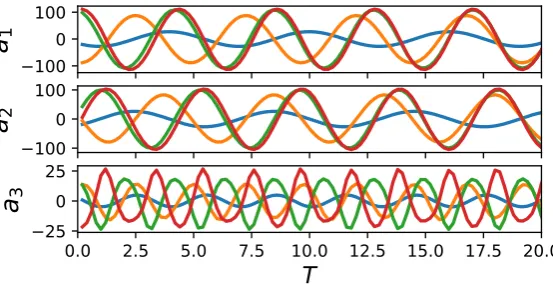
In this section, we explore sparse reconstruction of unsteady wake flows with well-developed periodic vortex shedding behavior. The GPOD type algorithm is chosen over the traditional Compressive sensing-based SR formulations to bypass the need for maintaining a separate measurement matrix, especially when employing point sensors to mimic realistic data acquisition. The first three POD modes and coefficients are computed and shown in figure5and6, respectively. Similar to the velocity field visualized in figure 4, the dominant POD modes (mode 1 and mode 2) capture the symmetric vortex shedding patterns at various length scales for all the cases. The vestiges of onset of instability at higher Re numbers (Re = 1000) is observed from the asymmetry in mode 3. This is consistent with the observations in [71], where the laminar vortex shedding happens at around Re = 47, and becomes unstable at ∼ 190 which deforms the small-scale structures at higher POD modes. On the other hand, the temporal evolution of POD coefficients show periodic limit-cycle behavior for all the
Renumbers with the characteristic frequencies increasing withReas shown in fig.6. The dependence of sparse reconstruction performance on Re is beyond the scope this article although we expect the system dimensionality to increase withReas the shear layers become thinner and consequently, require increased spatial sampling to capture all the relevant scales of motion. Instead, in this work we operate with narrower focus, i.e., explore and quantify how sparse reconstruction performance (in terms of error metrics) depend on sensor quantity, their placement and model dimensionality. With this in mind, we focus the analysis in the rest of the paper to a single Reynolds number, Re = 100. In this study, we choose 300 snapshots of data corresponding to a Reynolds number, Re = 100, corresponding to a non-dimensional time (T = U tD) of T = 60 with uniform temporal spacing of dT = 0.2s. T = 60 corresponds to multiple (≈10−15) cycles of periodic vortex shedding behavior.
(a)Re= 100 (b) Re= 1000
Figure 5. Isocontours of the three most energetic modes (from left to right) for the cylinder flow atRe= 100andRe= 1000.
100
0
100
a
1
100
0
100
a
2
0.0
2.5
5.0
7.5 10.0 12.5 15.0 17.5 20.0
T
25
0
25
a
3
Figure 6. Time evolution of the first three POD coefficients (Top: a1; Middle: a2; Bottom:
a3) for the cylinder flow at different Re number (Re = 100 (Blue), 300 (Orange), 800
(Green),1000(Red)) in the periodic vortex shedding regime.
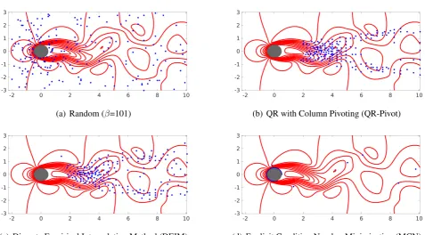
3.1.2. Smart Sensor Placement in Cylinder Wake
(a) Random (β=101) (b) QR with Column Pivoting (QR-Pivot)
(c) Discrete Empirical Interpolation Method (DEIM) (d) Explicit Condition Number Minimization (MCN)
Figure 7.Sensor locations learned form different choices of methods considered in this work including both random as well as smart algorithms for the cylinder wake flow (Re= 100). These image show the most relevant200sensors, i.e. (P = 200).
predicted on the cylinder surface. This is potentially indicative of the low-dimensional characteristic of the wake flow where only a few POD modes are needed to capture a significant portion of the energy.
4. Sparse Reconstruction of Canonical Fluid Flows
In this section, we explore sparse reconstruction of cylinder wake flow atRe= 100using the above SR infrastructure based on the GPOD formulation as against the traditional SR formulation. This choice is purely a matter of convenience and helps bypass the need for maintaining a separate measurement matrix (resulting in memory savings). In all the oversampled cases reported in this section, Tikhonov regularization is employed to reduce overfitting.
4.1. Sparse Reconstruction (SR) Experiments and Analysis
this approach in order to focus on assessing the relative roles of system dimensionality (K), sensor sparsity (P) and sensor placement (C) for the POD-based SR. In particular, we aim to accomplish the following through this study: (i) check if oversampling relative to desired system dimension (P > K) is sufficient condition for accurate reconstruction of the fluid flow for this POD-basedl2 reconstruction;
(ii) understand how sensor placement impacts reconstruction quality for different choice of basis. To learn the data-driven POD basis we employ the method of snapshots [52] as shown in eqns. (9)-(12). For the numerical experiments described here, the data-driven basis and coefficients are obtained from the full data ensemble, i.e.,M = 300snapshots corresponding toT = 60non-dimensional times. This gives rise to at most M basis for use in the reconstruction process in eqn. (3), i.e. a candidate basis dimension of Nb = M. As shown in table 1, the choice of algorithms depend on
the choice of system dimensionality (K), data sparsity (P) and dimension of the candidate basis space,
Nb. Recalling from the earlier discussion in section2, we see thatP ≥ K would require anl2 method
for a desired reconstruction sparsity K as long as P ≥ Nb. In case of POD-based SR, the basis are
energy optimal for the training data and hence, contain built-in sparsity. That is, as long as the basis is relevant for the flow to be reconstructed, retaining only the most energetic modes (basis) should generate the best possible reconstruction for the given sensor placement and quantity. Therefore, the POD basis need to be generated once and the reconstructed system dimension is determined by just choosing to retain the first few modes in the sequence. For generic basis with no built-in ordering of when using a library of basis with no clear classification available a priori, one requires to search for the K most significant basis amongst the maximum possible dimension of Nb = M using sparsity promoting l1
methods. l1 methods such as the iterative thresholding algorithms [27,72] require multiple solutions of
the least-squares problem before a sparse solution is realized. This results in necessary, but increased computational cost.
4.2. Comparison ofl2andl1Sparse Reconstruction using Energy-ordered POD Basis
In this subsection, we verify the equivalence betweenl2 reconstruction using energy ordered POD
basis and sparsity promotingl1−minimization reconstruction for the cylinder wake data when presented
the same sparse sensor data. The success of this verification will imply that the chosen POD basis ordered in terms of energy of the training data is also relevant to the data being reconstructed and also validate the accuracy of ourl1implementation. In such cases, choosing theK-most relevant basis for reconstruction
is trivial (and efficient) as one chooses the first or last K modes (as against searching for the sparsest
K modes usingl1) as the candidate basis forl2 reconstruction provided sufficient sparse data,P > K,
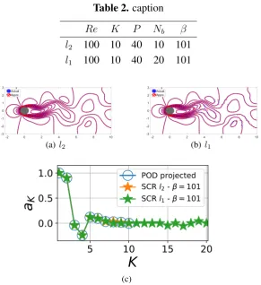
is available. To verify this, we consider two cases of reconstruction for the limit-cycle cylinder wake at Re = 100. Case (a): P > K, K = Nb and using least squares reconstruction; Case (b): P > K,
K < Nb ≤ M and employs l1 reconstruction using optimal matching pursuit. Figure 8 and table 2
compares the reconstructed fields and the K predicted weights for the two cases for a single snapshot corresponding toT = 0.2. In this study we use a greedy optimal matching pursuit algorithm for thel1
norm minimization, CoSAMP as described by Needell and Tropp in [11].
Table 2. caption
Re K P Nb β
l2 100 10 40 10 101
l1 100 10 40 20 101
(a)l2 (b) l1
5
10
15
20
K
0.0
0.5
1.0
a
K
POD projected
SCR l
2- = 101
SCR l
1- = 101
(c)
Figure 8. Comparison of the sparse reconstruction using both l1 and l2 minimization
methods for basis that is ordered in terms of energy content. The reconstructed and actual flowfields atT = 0.2are compared in (a) forl2and (b)l1. The corresponding POD features
from both methods are shown in (c).
when the relevance of sparse data to the candidate basis space is unclear. For the rest of this paper, we will leverage energy hierarchy of the candidate POD basis and adopt the SR problem formulation using al2 minimization algorithm withK =Nb. In other words, the candidate basis space is chosen based on
the desired reconstructed field dimension and not fixed.
4.3. Sparsity and Energy Metrics
For this SR study, we explore the conditions for accurate recovery of information in terms of data sparsity (P) and system sparsity (K) which also represents the dimensionality of the system in a given basis space. In other words, sparsity represents the size of a given basis space needed to capture a desired amount of energy. As long as the measurements are incoherent with respect to the basis Φ
and the system is overdetermined, i.e., P > K, one should be able to invert Θ to recover the higher dimensional state,X. From earlier discussions in section2, we knowP > K is a sufficient condition for accurate reconstruction using l0 minimization. Thus, both interpretations require a minimum quantity
of sensor data for accurate reconstruction and is verified through numerical experiments in section 4.4. In this section, we describe how the different system sparsity metrics, K = Nb, are chosen for the
0
2
4
6
8
10
12
50
100
K
(%)
Re100Re300 Re800Re1000 KK= 95%= 99%
0
2
4
6
8
10
12
K
95
100
K
(%)
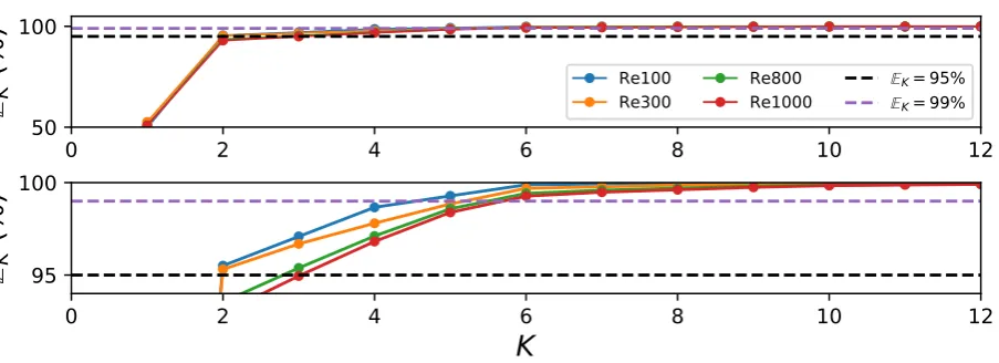
Figure 9. Schematic shows the cumulative energy capture corresponding to various system sparsity levels, K, (i.e. the number of POD modes) for cylinder flow at Re = 100 to 1000. The bottom figure is a magnified version of the top figure for EK. For Re =
100,300,800,1000:K95 = [2,2,3,4]andK99 = [5,6,6,6], respectively.
For POD one easily defines a cumulative energy fraction captured by theK most energetic modes,EK,
using the corresponding singular values of the data as shown in eqn. (29).
EK = K
X
k=1
λk
(λ1+λ2+...+λM)
×100. (29)
In the above, the singular values, λ are computed from eqn. (10), and M is the total number of possible eigenvalues for M snapshots. As a result, the energy fraction EK corresponding to sparsity
K for the different flow Reynolds numbers, Re, is shown in Figure 9. For the cylinder flow case with Re = 100, one requires two and five POD modes to capture 95%and 99%of the energy content respectively, indicative of the low dimensional dynamics. We denote the mode numbers corresponding to 95% and 99% of the energy capture as K95 and K99 respectively. In this case, we compute
errP ODK =
X−ΦP OD1..K aP OD1..K
2, where Φ
P OD
1..K , and aP OD1..K represent the matrix comprising of K
POD bases and the corresponding coefficients for the different snapshots respectively. To assess SR performance across different flow regimes (that have differentK95) with different values ofK we define
a normalized system dimension, K∗ = K/K95 and a normalized sensor sparsity, P∗ = P/K95. This
allows us to design an ensemble of numerical experiments in the discretized P∗ −K∗ space and the outcomes can be generalized beyond the current study. In this work, the design space is populated over the range 1 < K∗ < 6and 1 < P∗ < 12for POD-based SR withK bounded by the total number of snapshots,M = 300. The lower bound of one is chosen such that the minimally accurate reconstruction captures 95% of the energy. If one desires a different reconstruction norm, then K95 can be changed
to Kxx without loss of generality and the corresponding K-space modified accordingly. Alternately,
one can choose EK, the normalized energy fraction metric to represent the desired energy capture as a
To quantify thel2reconstruction performance, we define the mean squared error as shown in eqn. (30)
below,
SRK∗,P∗ =
1 M 1 N M X j=1 N X i=1
(Xi,j−X¯i,jSR)
2, (30)
whereXis the true data, andX¯SRis the reconstructed field from sparse measurements as per algorithm3.
N and M represent the state and snapshot dimensions and related to indices i and j, respectively. Similarly, the mean squared error F R
K∗
95 and
F R
K∗ for thefull reconstructionfrom the POD basis can be
computed as:
F RK∗
95 = 1 M 1 N M X j=1 N X i=1
(Xi,j −X¯ F R,K95∗ i,j )
2, (31)
F RK∗ =
1 M 1 N M X j=1 N X i=1
(Xi,j−X¯F R,K ∗ i,j )
2,
(32)
whereX¯F R is the full field reconstruction using exactly computed POD coefficientsa. For POD this is
simplya=ΦTXas per eqn. (12). K95∗ is the normalized system dimension (i.e. number of POD modes normalized by K95) corresponding to 95% energy capture and K∗ = K/K95 represents the desired
reconstructed system dimension. Note thatK95∗ =K95/K95 = 1is trivially seen to be one for this case.
Using the above definitions, we can now generate normalized versions of the absolute (1) and relative
(2) errors as shown in eqn. (33). 1 represents the SR error normalized by the corresponding full
reconstruction error for 95% energy capture. 2 represents the normalized error relative to the desired
reconstruction accuracy for the chosen system reconstruction dimension,K. These two error metrics are chosen so as to achieve the twin goals of assessing the overall quality of the SR in a normalized sense (1) and the best possible reconstruction accuracy for the chosen problem set-up (i.eP, K). Thus, if the
best possible reconstruction for a given K is realized then2 will take the same value across different
K∗. This error metric is used to assess relative dependence ofP∗ onK∗ for the chosen flow field. On the other hand, 1 provides an absolute estimate of the reconstruction accuracy for a given flow system
so that minimal values ofP∗, K∗needed to achieve a desired accuracy can be identified.
1 =
SR K∗,P∗
F R K∗95
, 2 =
SR K∗,P∗
F R K∗
. (33)
4.4. Sparse Reconstruction of Cylinder Wakes
(a)1(Maximum error) (b) 2(Maximum error)
(c) 1(Minimum error) (d) 2(Minimum error)
(e) 1(Average error) (f) 2(Average error)
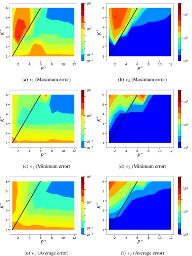
Figure 10. Isocontours of the normalized mean squared POD-based sparse reconstruction errors (l2norm) corresponding to the sensor placement with maximum and minimum errors
from the chosen ensemble of random sensor arrangements. The average error across the entire ensemble of ten random sensor placements is also shown. Left: normalized absolute error metric,1. Right: normalized relative error metric,2.
4.4.1. Sparse Reconstruction Accuracy
By computing the errors as described in section4.3 across the K∗ − P∗ space, the contours of1
and2 are generated for both the random as well as greedy sensor placements in figures10and 11. As
(a) 1(QR with column pivoting) (b) 2(QR with column pivoting)
(c) 1(DEIM) (d) 2(DEIM)
(e) 1(MCN) (f) 2(MCN)
Figure 11. Isocontours of the normalized mean squared POD-based sparse reconstruction errors (l2 norm) corresponding to the different greedy sensor placement methods. Left:
normalized absolute error metric, 1. Right: normalized relative error metric, 2. (MCN:
Minimum Condition Number)
of sensor locations corresponding to different seeds (as denoted by β in this article). Specifically, we compute the SR errors from ten different random seeds and the corresponding reconstruction errors are presented in terms of the mean, maximum and minimum (based on the average over theK∗−P∗ space) in fig. 10. For the greedy ‘smart’ sensor placements a single realization is representative of the method and corresponding error contours for1and2are shown (fig.11). For ease of interpretation, the contour
The relative error metric 2 (the right column in Figure 10 and 11), shows that the smaller errors
(predominantly blue regions) are located in the region where P∗ > K∗ and approximately separated from the rest of the K∗ −P∗ space using a black diagonal line. This indicates that the oversampled SR problem with P > K, i.e. having more sensors than the dimensionality chosen to reconstruct the system yields good results in terms of 2 while for small P∗, the normalized relative error can reach
as high as O(101 −102). Since
2 is normalized by the error contained in the exact K-dimensional
POD reconstruction, this metric represents how effectively the sparse sensor data can approximate the
K-dimensional solution usingl2minimization for the given sensor quantity and placement. In principle,
the exactK-sparse POD reconstruction is the best possible outcome to expect irrespective of how much sensor data is available as long asK =Nb. Another way of looking at this is that by constraining the SR
problem by choosing a relevant POD basis with knowledge of the energy hierarchy, thel2reconstruction
approaches thel0 minimization solution, i.e. theK-sparsest basis are selected by default. Of course, this
is not feasible in practical situations where the basis relevance (and its ordering) to the data is not known
a priori. We also observe that as expected 1 contours adhere to aL-shaped structure indicating that
absolute normalized error reduces as bothP andK increase due to oversampling and increased system dimension. In practice, 1 is the more useful metric for planning and designing the sparse recovery
framework for a given flow system, provided the system dimension, i.e. K95orKxx is known.
While qualitatively accurate reconstruction is almost always observed for the higher values ofP∗ and
K∗for the different sensor placements, there appear to be exceptions in the form of higher reconstruction errors even when P∗ > K∗. This is observed for both the random sensor placement as well as smart sensing approaches. In fact, for the random sensor placement method, a small portion of 2 in the
region abutting the P∗ = K∗ line shows nearly an order of magnitude higher error, O(101) (colored
as yellow in Figure 10) as compared to rest of the region with expected values of O(1). This trend is observed for the greedy sensor placement methods as well, particularly QR-pivoting and MCN. In general, the greedy sensor placement methods show better reconstruction performance when compared to random approaches in the regions surroundingP∗ ≈K∗. This is not surprising given that oversampled (P∗ K∗) or under-sampled (P∗ K∗) reconstruction will invariably generate low and high errors respectively. It is only when operating in the transition region that separates under-sampling from over-sampling that sensor placement becomes important.
4.4.2. Assessment of Sensor Placement
Among the three greedy sensor placement methods experimented in this work, DEIM provides the most reliable reconstruction (fig.11(c,d)) and closely followed by QR factorization with column pivoting (fig. 11 (a,b)). MCN method which explicitly minimizes the condition number of M shows good reconstruction accuracy for smaller values of K∗ until about K∗ ∼ 4 − 5 (see fig. 11 (e,f)). The anomalous inaccuracy that is observed for reconstruction dimensions beyond K∗ ≈ 5 is due to very few sensors being generated in the wake downstream of the cylinder as seen in fig.7(d). For this fluid flow, the dominant dynamics occur in the wake and MCN produces very few sensors in this region which under-samples the flow field for higher dimensional reconstruction.
1 2 3 K 4 5 6 0 10 20 aK POD projected SR l2 ( =101)
1 2 3 4 5 6
K 0 10 20 aK POD projected SR l2 (QR-Pivoting)
1 2 3 4 5 6
K 0 10 20 aK POD projected SR l2 (DEIM)
1 2 3 4 5 6
K 0 10 20 aK POD projected SR l2 (MCN)
(a)K∗= 1
1 2 3 K 4 5 6
0 10 20
aK
POD projected SR l2 ( =101)
1 2 3 4 5 6
K 0 10 20 aK POD projected SR l2 (QR-Pivoting)
1 2 3 4 5 6
K 0 10 20 aK POD projected SR l2 (DEIM)
1 2 3 4 5 6
K 0 10 20 30 aK POD projected SR l2 (MCN)
(b) K∗= 2
1 2 3 K 4 5 6
0 10 20
aK
POD projected SR l2 ( =101)
1 2 3 4 5 6
K 0 10 20 aK POD projected SR l2 (QR-Pivoting)
1 2 3 4 5 6
K 0 10 20 aK POD projected SR l2 (DEIM)
1 2 3 4 5 6
K 0 10 20 aK POD projected SR l2 (MCN)
(c) K∗= 3
Figure 12. 1strow (Randomβ = 101),3rdrow (QR-Pivot),5throw (DEIM) and7th(MCN)
row: we show the line contour comparison of streamwise velocity between the actual CFD solution field (blue) and the POD-based SR reconstruction (red) forRe = 100 atP∗ = 10 and K∗ = 1,2,3. 2nd row (Random β = 101), 4th row (QR with column pivoting), 6th
row (DEIM) and8throw (MCN) show the corresponding projected (full reconstruction) and