How Does the Share of Imports Change During Structural Adjustment?

Menzies Building

Monash University Wellington Road

CLAYTON Vic 3168 AUSTRALIA

Telephone:

(03) 9905 2398, (03) 9905 5112

from overseas:

61 3 9905 5112

Fax numbers:

from overseas:

(03) 9905 2426, (03) 9905 5486

61 3 9905 2426 or

61 3 9905 5486

e-mail

[email protected]

H

OW DOES THE

S

HARE OF

I

MPORTS

C

HANGE

D

URING

S

TRUCTURAL

A

DJUSTMENT

?

by

A

lan

A

.

P

OWELL

Monash University

Preliminary Working Paper No. OP-86 June 1996

ISSN 1 031 9034 ISBN 0 7326 0738 8

The Centre of Policy Studies (COPS) is a research centre at Monash University devoted to quantitative analysis of issues relevant to Australian economic policy. The Impact Project is a cooperative venture between the Australian Federal Government and Monash University, La Trobe University, and the Australian National University. COPS and Impact are operating as a single unit at Monash University with the task of constructing a new economy-wide policy model to be known as MONASH. This initiative is supported by the Industry Commission on behalf of the Commonwealth Government, and by several other sponsors. The views expressed herein do not necessarily represent those of any sponsor or government.

C

ENTRE

of

P

OLICY

S

TUDIES

and

the

I

MPACT

Estimating the price responsiveness of market shares during a

period of structural transition requires a distinction to be made

between responses to variables explicitly recognized in the model

and those due to more general changes in the trading

environ-ment. Often the latter are minimally modelled as market

penetration curves taking the form of a sigmoid trend. Broadly

this is the approach followed in the present paper; however, the

trend ‘parameter’ capturing ultimate market share at a fixed level

of price competitiveness is itself made a logistic function of the

relative price variable measuring such competitiveness.

The application of the model is to quarterly data on the share of

imports in Australian personal consumption over the 1980s and

the first half of the 1990s. Most of the signal relevant to price

competition between domestic and imported consumer goods

occurred over the four years 1985

−

1988. This coincided with

sizeable movements in the real exchange rate; and therefore,

presumably, with collinear movements in the prices of the

components within the domestic and the imported aggregates,

which would be favourable circumstances for the application of

Hicks’ composite commodity idea. The responses in aggregate

market shares during this episode suggest a very long-run

Armington elasticity in the range 3.4 to 4.8, with short-run

(quarterly) values of 0.6 to 0.8.

Keywords: import substitution, Armington elasticity,

consumption, structural adjustment, logistic function, market

penetration curve.

iii

A

1

I

2

T

D

L

M

2.1 The problem 3

2.2 Price Responsiveness of the ceiling

Value of Imports’ share 3

2.3 Market Adjustment Through Time 

Non-stochastic Dynamics 4

3

E

M

3.1 Restricted maximum likelihood estimator 7

3.2 Error correction 8

3.3 Stochastic specification 9

3.4 Objective function 10

3.5 Side constraints 10

4

T

D

5

R

5.1 Estimates under the autoregressive hypothesis H_A 11

5.2 Estimates under the moving-average hypothesis H_B? 17

5.3 Interpretation of results, I − the bad news 17

5.4 Interpretation of results, II − the good news 18

5.5 Interpretation of results, III −

short-run price substitutability 18

6

N

D

R

, R

E

P

-

T

6.1 The bad and the good news revisited 25

6.2 Summary of estimation results 28

7

C

R

7.1 Scope for further work 29

7.2 Prospects for market penetration by imports 29

iv

Table 5.1 Restricted Maximum Likelihood Estimates of the Double

Logistic Model fitted in the First Differences under

Hypothesis H_A− Quarterly Data, 1980Q3-1993Q1 12

Table 5.2 Constraint Binding on Parameter Solution Presented

in Table 5.1 13

Table 6.1 Estimates of the Double Logistic Model fitted in First

Differences under Hypothesis H_A− Quarterly Data,

1981Q3-1995Q4 21

Table 6.2 Estimates of the Double Logistic Model fitted in the First

Differences under Hypothesis H_A with Price Sensitivity

set to Zero − Quarterly Data, 1981Q3-1995Q4 24

LIST OF FIGURES

Figure 1.1 Market penetration curve 1

Figure 1.2 Share of imports in consumption and competitiveness

index 1980Q3 through 1993Q1 2

Figure 2.1 Decline in ultimate import penetration as Australia’s

competitiveness increases 4

Figure 5.1 Actual and fitted values of the ratio transform of

imports’ market share, 1980Q3−1993Q1 13

Figure 5.2 Projected and actual shares of imports in consumption,

1980Q3−1993Q1 14

Figure 5.3 Projected and actual changes in shares of imports in

consumption 1980Q3−1993Q1 14

Figure 5.4 Projected and ‘actual’ values of ∆ log L from equation

(3.9), 1980Q3−1993Q1 15

Figure 5.5 Residuals from the fitted equation (3.9), 1980Q3−1993Q1 15

Figure 5.6 Fit of the model, 1980Q3−1993Q1, when price

influences are removed (i.e., when γ = 0) 16

Figure 5.7 Estimated values of imports’ ultimate share of consumption

at levels of competitiveness that obtained during the

v

between imported and domestically produced

consumption goods, 1980Q3−1993Q1 19

Figure 6.1 Data on imports’ share in consumption on old and new basis,

with projections from old estimates on new basis,

1993Q2-1995Q4 19

Figure 6.1 Data on imports’ share in consumption on old and new basis,

with projections, 1983Q2−1995Q4 19

Figure 6.2 Data on competitiveness on old and new basis 20

Figure 6.3 Projected and actual shares of imports in consumption,

1981Q3−1995Q4 (fitted values from Table 6.1 estimates) 22

Figure 6.4 Projected and actual changes in shares of imports in

consumption, 1981Q3−1995Q4 (fitted values from

Table 6.1 estimates) 22

Figure 6.5 Fit of logarithmic changes in the log-ratio transform, ∆ ln L,

1981Q3−1995Q4 (fitted values from Table 6.1 estimates) 23

Figure 6.6 Residuals from fitted equation (3.9), 1981Q3−1995Q4

(fitted values from Table 6.1 estimates) 23

Figure 6.7 Projected and actual shares of imports in

consumption, 1981Q3−1995Q4, when price

influences are removed (i.e., when γ = 0) 25

Figure 6.8 Estimated values of imports’ ultimate share of consumption

at levels of competitiveness that obtained during the sample,

1981Q3−1995Q4 (new data, Table 6.1 estimates) 26

Figure 6.9 Projected trajectories of imports’ share in consumption

according to estimated parameters shown in Tables 5.1, 6.1 and 6.2 when Australian competitiveness remains

at its 1995Q4 value 27

Figure 6.10 Projected trajectories of imports’ share in consumption according to estimated parameters shown in Tables 5.1 and 6.1 when Australian competitiveness increases or

deteriorates by 4 per cent per annum 27

Figure 6.11 Projected trajectories of imports’ share in consumption according to estimated parameters shown in Tables 5.1 and 6.1 when Australian competitiveness increases or deteriorates by 4 per cent per annum, with seasonal

DURING STRUCTURAL ADJUSTMENT?

by

Alan A. POWELL*

Monash University

1. Introduction

Recent years have seen increasing market penetration by imports in several areas of the economy. If we regard this experience as reflecting mainly changes in Austra-lian competitiveness – in other words, if we follow the Armington paradigm as imple-mented by Alaouze et al. [1] – we may come to the conclusion that substitution elas-ticities between domestic and foreign goods are very high, and therefore that even a slight deterioration in our competitiveness could lead to the annihilation of domestic import competing industries.

Is there an alternative view? This depends on how one interprets the current phase of global trading history. If the extensive relocation of production for manufac-tures in developing countries (especially in Asia) is seen as the movement from one equilibrium trading pattern to another, then the long-term outlook for Australia's import competitors may not be so grim. Whilst rapid displacement by imports may be occurring now, this could correspond to the rapid growth segment "A" of the market penetration curve shown in Figure 1.1.

K_t

τ

t

Market share of "new" (read "imported") goods on the assumption that local competitiveness remains constant at its value at time t

time

Wτ

ceiling

K _t ≤ 1

A

Figure 1.1 Market penetration curve. Note that a lowered competi-tiveness of local suppliers would lead to a higher ceiling on imports' final share of the market.

If the above view is accepted, then, as hazardous as all such exercises are, it leaves little alternative but to attempt to estimate the dynamics of the adjustment path.

Some circumspection should accompany this exercise. As is obvious from Figure 1.1, if all sample data were to occur in the segment "A", and if there was relatively little time-series variation in competitiveness, then the location of the ceiling K_t would either be unidentified, or else determined largely by second-order parameters of the penetration curve. It is unlikely that we would be able, under the postulated conditions, to estimate such parameters with precision.

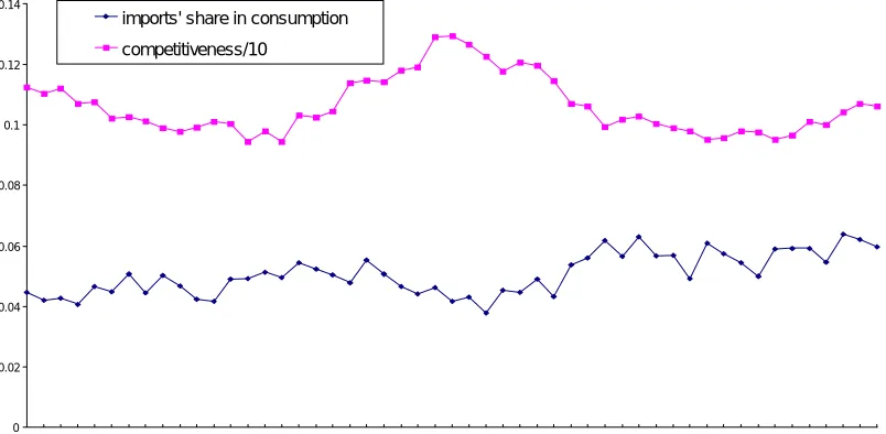
In fact in recent years there has been substantial variation both in competitive-ness, and in market shares (at least for some major aggregates). In the balance of this paper the focus is on aggregate consumption in Australia. Imports' share (quantity index basis) and local competitiveness are shown in Figure 1.2. Given the variation evident in these data, it does seem worthwhile to attempt to disentangle the dynamics of market share adjustment from price responsiveness.

0 0.02 0.04 0.06 0.08 0.1 0.12 0.14

1 2 3 4 5 6 7 8 9 10 11 12 13 14 15 16 17 18 19 20 21 22 23 24 25 26 27 28 29 30 31 32 33 34 35 36 37 38 39 40 41 42 43 44 45 46 47 48 49 50 51 imports' share in consumption

competitiveness/10

Figure 1.2 Share of imports in consumption and competitiveness index 1980Q3 through 1993Q1

The remainder of this paper is structured as follows. Section 2 contains a model with the following features:

(i) Imports' 'market share'1 is a logistic function of time, with ultimate market penetration depending inversely on local competitiveness.

(ii) The ultimate market share of imports is itself a (displaced) logistic function of competitiveness.

Section 3 contains a discussion of the method used to estimate the model, while section 4 contains a brief discussion of the data. An initial set of results is given in Section 5. The implications for the performance of the model of a new data release are explored in Section 6, where a summary of the estimation results is also given. Finally, concluding remarks are offered in Section 7.

2. The Double Logistic Model

2.1 The problem

The problem posed above may be restated succinctly as: given time-series data on imports' market share in consumption – about 13 years of quarterly observations – estimate the penetration curve subject to a sensible role for "competitiveness" (here defined as the ratio of the purchasers' prices of imported consumption goods to the prices of domestically produced consumption goods). Ultimately we want to forecast the (time) change in market share as a function of time and of change in competitive-ness P_t ,where

P_t ≡ P_import(t)/P_domestic(t) .

For future reference, note p_t ≡ d ln P_t.

2.2 Price responsiveness of the ceiling value of imports' share

In the basic model it is assumed that relative prices enter market dynamics through the 'ceiling', or saturation–share, parameter, K:

(2.1) K_t = f(P_t) ; 0 ≤ K_t ≤ 1 .

Note (i) that K's dependence on time is solely via its dependence on competitive-ness, P_t; and (ii) that P_t in (2.1) is playing the role of the long-run expectation held at time t for future competitiveness. More elaborate developments of the theory sketched below would replace P_t in (2.1) by such an expectational variable.

The form of f(•) in (2.1) is taken to be a displaced logistic in the logarithm of P_t:

(2.2) K_t = θq(t) +

(1 – θq(t) )

1 + α_q(t) P_tγ

where q(t) is an indexing function which identifies the quarter of the year in which ob-servation t falls, and the parameters are θ₁, θ₂, θ₃, θ₄ (the minimum ultimate share possible for imports), α₁, α₂, α₃, α₄ (location parameters) and γ (sensitivity of the ultimate share of imports to competitiveness). Other than γ, the parameters are indexed by quarter to account for seasonality in import patterns. The expected signs of the θs, αs and γ are positive. In addition, the θ−parameters are constrained to lie

within the [0, 1] interval. A value of θ > 0 implies that even if Australian competitiveness were to become superb (Pt→ ∞), imports would still ultimately achieve

a share θ (albeit a small share) of the market.

In the derivations below it will be helpful to use a variable Q_t defined as

(2.3) Q_t = 1

1 + α_q(t) P_tγ

which is a pure logistic function with unit ceiling parameter. Then (2.2) may be rewritten as

(2.4) K_t = θ_q(t) + (1 - θ_q(t) ) Q_t

(2.5) ∂K_∂ t

v = (1 - θ) ∂Qt/∂v

and that

(2.6) ∂ ln K_∂ t

v =

(K_t - θ) K_t

∂ ln Q_t ∂v

where v is any parameter or variable, and where in omitting the q(t) subscripts on θ we have (for the time-being) neglected quarter-to-quarter changes due to the seasonal pattern in the θs. In particular,

(2.7) ∂

K_t

∂γ = – (1 - θ) γ αt Qt2 Ptγ−1 ,

and

(2.8)

d ln K_t

dt = – γ

(K_t - θ)

K_t (1 - Qt)

d ln P_t dt .

Notice that with γ > 0, (2.8) implies that the ultimate share of imports K_t is monotonic decreasing in Australian competitiveness P_t. This is illustrated in Figure 2.1.

Imports’ ultimate market share

K

first quarter response curve

θ1 θ

2

imports’ minimum possible ultimate market share in quarter 1

second quarter response curve

imports’ minimum possible ultimate market share in quarter 2

Log of competitiveness ln (P_t )

Figure 2.1 Decline in ultimate import penetration as Australia's competitiveness increases. Note that there is a different curve for each quarter, and possibly a finite positive lower bound on imports' ultimate market share which is quarter-specific.

2.3 Market adjustment through time — non-stochastic dynamics

With price-competition modelled via (2.2), a second logistic function is now intro-duced to model the sigmoid trend in market penetration shown in Figure 1.1:

(2.9) W_t =

K_t

where W_t is the share of imports (quantity basis) in total sales to consumption, and a and b are parameters with expected signs which are positive and negative respectively.2

The change over an interval of time dt in imports' market share can be found from:3

(2.10) d ln

(K_t - W_t)

W_t = b dt .

Using w_t and k_t to denote d ln K_t and d ln W_t respectively, (2.10) may be expressed as:

(2.11) w_t = k_t -













K_t - W_t

K_t b dt .

If K is fixed, (2.11) implies that the logarithmic time rate of change of market share is directly proportional to the gap between the ceiling and the current share, where this gap is expressed as a fraction of the ceiling value, the constant of proportionality being (-b). For shares which grow with time it follows that b is negative.

To simplify matters while ideas are clarified, we drop the seasonal variation in the θs and αs for the moment. Taking total differentials of (2.4) we obtain:

(2.12) k_t =













K_t - θ

K_t qt ,

where q_t ≡ d ln Q_t. Using (2.8) we obtain

(2.13) k_t = – γ

(K_t - θ)

K_t (1 - Qt) pt .

Substituting (2.13) into (2.11), we find

(2.14) w_t = – γ













K_t - θ

K_t (1 - Qt) pt – b

_











K_t-W_t K_t dt .

[term 1] [term 2]

Consider a period in which competitiveness is rising (p _t > 0). Since α, γ > 0, b < 0 and K ≥ W, we see that the proportional change w_t in the share of imports at time t consists of two parts: a fall due to the effect of increased competitiveness (term 1) and a rise due to the working through of market penetration (term 2). The first effect becomes positive if competitiveness falls; the second is always positive.

2 Note that we do not require W_t to approach θ as t → – ∞_{; in fact, Wt} → 0 as t → – ∞. This is interpreted to mean that zero is the natural origin for foreign market share before the structural shift in trading patterns.

Let M_t and Y_t denote imported and domestic 'quantities' (i.e., $A of a base period). Then by definition we have

(2.15) W_t ≡ M_t / (M_t + Y_t)

and

(2.16 ) w_t ≡ (1 - W_t) (m_t - y_t) = (1 - W_t) d ln













where m_t and y_t respectively are d ln M_t and d ln Y_t.

Consider a fixed point of time and allow a change in competitiveness (in the sense of a deviation from control at t). From (2.14) and (2.16) we see that the elasticity of substitution between imports and the domestic good is4

(2.17) σ_SR = –

























Y_t ÷ d ln

_











P_domestic



= γ













K_t (1 - Qt) / (1 - Wt) = γ

_











K_t

(1 - K_t)

(1 - θ) / (1 - Wt) .

Above σ carries subscripts SR to denote that it is a short-run value. In the long run, as t → ∞, Wt → K_t,and wehave for the long-run substitution elasticity (at fixed P_t):

(2.18) σ_LR = γ (K_t - θ) / {K_t (1-θ) } .

Since W_t ≤ K_t, σ_LR ≥ σ_SR. Notice that "long-run" in this case means that we compare the displacement between two situations in which market saturation conditional on P_t has occurred. Also notice that, as θ → 0, σ_LR → γ, which justifies the description of γ as the long-run sensitivity of imports' market share to local competitiveness, more briefly referred to below as the price sensitivity parameter.

3. Estimation of the Model

The approach to estimation of the model is to list the desirable properties of the estimator, and to incorporate each, either within the objective function, or as a set of side constraints.

The properties considered desirable were the following:

(1a) The estimated model must never forecast a value of the share of imports that exceeds 1 or is less than zero.

(2a) If possible, the stochastic specification should be similarly constrained so that a realization of Wt outside the [0,1] interval is impossible.

(3a) _{The fitted { Wt } must provide within-sample unbiased estimates of the actual} { Wt } in the sense that the sample regression of the actual share Wt on fitted values of this variable must be a straight line through the origin. (In the linear model, this is a property of OLS estimates.)

(4a) The fitted {∆_{Wt} must be similarly unbiased, so that the sample regression of the} actual changes in share ∆_{Wt on fitted values of this variable must also be a} straight line through the origin.

(5a) The serial properties of the fitted equation must be satisfactory; in particular:

I. The right and left-hand sides of the fitted equation should pass at least informal tests of cointegration.

II. The first-order serial correlation of the residuals should be close to zero (with a Durbin-Watson statistic between 1.8 and 2.2, say). (Misspecification of seasonality would likely lead to violation of this requirement.)

III. Serial correlation between observations realized in the same season must be eliminated (with a 4th-order Durbin-Watson statistic between 1.8 and 2.2, say).

Subject to all of the above, the likelihood of the sample data should be maximized with respect to the parameters finally chosen.

The above requirements are incorporated into estimation as follows.

(1b) _{The logistic function (2.9) returns values of Wt which lie in (0, Kt] for t in the} interval (-∞, ∞_{), while the function (2.2) guarantees that Kt is bounded in} (0, 1) provided that θ_{q(t) is similarly bounded for each of its four possible} values. We enforce the latter constraint in estimation. Using (2.9) as a fore-casting equation will then satisfy (1a).

(2b) The requirement (2a) can be met by transforming the model using the log-ratio form (Fry, Fry and McLaren [1996].5

(3b) Requirements (3a), (4a) (5a)II and (5a)III are to be enforced directly in the estimation as side constraints on the optimization of the fit.

(4b) Requirement (5a)I is to be met by allowing for an error-correction mechanism in the fitted equation, and by visually checking the reversion to mean of the fitted equation.

(5b) Finally, the objective function is chosen to be the error sum of squares of the log-ratio transform of the model with error correction included. Under normality of the equation errors, the likelihood is maximized subject to the explicit constraints listed above.

3.1 Restricted maximum-likelihood estimator

It is assumed that the model is to be used to predict both the level and the quarterly changes in imports' market share, ∆W₁, ..., ∆W₅₀. Conditional on competitiveness P_t, the date t, and the parameters {θ₁, θ₂, θ₃, θ₄

α

α

α

α

γ

By construction, the W^_t lie in the interval [θq(t), Kt]. It follows that the variable

(3.1) V^_{t =} W

^

t – θq(t)

K_t – θ_q(t)

satisfies the constraint

(3.2) 0 < V^_t < 1 .

Notice that if Wt indicates actual share data and Vt is defined by,

(3.3) V_{t =}

W_t – θ_q(t)

Kt – θq(t)

then, for arbitrary K_t it cannot be guaranteed that

(3.4) 0 < V_t < 1 ;

however, if K_t is restricted to be greater than the largest W_t observed in the sample, (3.4) will necessarily hold. It turns out that our estimates below respect the inequality

(3.5) K^t > Max

t ∈_sample

{

} .

Application of the log-ratio transform (Fry, Fry and McLaren [1996]) to this model involves forming the variables

(3.6a) L^_t = V^_{t /(1 –} V^_{t )}

and

(3.6b) L_t = V_{t /(1 –} V_{t ) .}

The basic idea underlying this transform is to map the variables V_t and V^_t, which both are defined on the closed unit interval [0, 1] onto the real line (-

∞

,

∞

(3.7) ln L_t = ln L^_t + v_t , or in the differences as

(3.8) ∆ ln L_t = ∆ ln L^_t + u_t , [∆(•)_t ≡ (•)_t+1 - (•)_t ]

where vt and ut are zero-mean random errors (with ut ≡ ∆ vt). Under the conditions

postulated above, the values of W_t estimated from (3.7) are guaranteed to remain in the [0, 1] interval, while the domain of variation of ut remains unrestricted.

Given the widespread problem of high serial correlation, it used to be common to choose the difference form of the equation for estimation; the critique of the cointegrationists that such a procedure throws away the long-run relationship of interest latterly has caused empirical workers to think twice about differencing.

So far as the current paper is concerned, this part of the critique clearly is not applicable, since the parameters of the long-run relationships imbedded in {(2.3), (2.4), (2.9)} are recoverable from the estimation of either (3.7) or (3.8). The argument against first differencing must then proceed in terms of efficiency of estimation, rather than lack of identification.

3.2 Error correction

assess whether the process as modelled in (3.8) is successful is ensuring that the estimated process reverts to mean. If this is the case, the ECM should have a coeffi-cient close to zero (which can be checked from the estimates). For this reason we replace (3.8) for estimation purposes by:

(3.9) ∆ ln L_t = ∆ ln L^_t + ψ ln

(

)

Alternatively, we can think of (3.9) as the Cochrane-Orcutt transform of (3.7) with autoregressive parameter ρ ≡ 1 – ψ. Even if ψ = 0, V^

t and Vt may remain cointegrated

in the sense that the internal logistical structure imbedded in both may stop them drifting apart over time.

A more compact notation for (3.7) and (3.9) is:

(3.10) Y_t = Xt + vt ,

and

(3.11) y_t = x_t + ψ

(

)

in which the variables x and X are functions of the data and the parameters of the model (with X = ln L^, Y = ln L, x = ∆ ln X and y = ∆ ln Y). Note that the dependency of y and Y on data is via realizations of the endogenous variable W_t only, whereas that of x and X is via exogenous variables only.

3.3 Stochastic specification

We assume throughout that the errors v and u in (3.7) and (3.8) have zero means. If v follows a first-order Markov scheme (i.e., is AR(1)) with a first-order serial correlation equal to (1 - ψ), then (3.9) is the appropriate equation for estimation and should yield a Durbin-Watson statistic close to 2. On the other hand, if v is close to being serially uncorrelated, then (3.7) is the appropriate estimating equation and should yield residuals with a DW close to 2; the errors u in (3.8), on the other hand, will follow a first-order moving average (MA(1)).

The small sample size (N=51) and the relatively large number of parameters (thirteen including the error variance) make it unlikely that powerful discrimination between

HA: vt ~ AR(1) & ut classically well behaved

and HB: ut ~ MA(1) & vt classically well behaved

would be possible were the model not so highly constrained. Below attempts are made to estimate the model under HA and under HB. Unlike the more conventional approach

to estimation, the maintained hypotheses are to be 'enforced' rather than tested. Thus under HA the objective function is to be optimized in that part of the parameter space

yielding diagnostics indicating freedom from serial correlation of the fitted uts; under

HB,optimization is to takeplaceinthe regionthatyieldsdiagnostics indicatingfreedom

fromserialcorrelationinthefittedvts.

3.4 Objective function

(3.12) φA =

Σ

t=1 51

u^_t2 ;

under HB, the objective function is

(3.13 ) φB =

Σ

t=1 50

v^_t2 .

In the last two equations, the hats (^) indicate the fitted values of the equation errors. Thus our estimator is based on (restricted) non-linear least-squares applied to (3.11) in the case of HA, and to (3.10) in the case of HB. Under normality of the error

distri-butions, these estimators (with minimands φA and φB) are restricted

maximum-likelihood estimators under their respective maintained hypotheses HA and HB.

3.5 Side constraints

Unrestricted maximum likelihood will find parameters that yield values of ∆W^_t that are biased estimates of ∆W_t even within the sample. This is avoided by imposing two side constraints on the minimization of (3.12); namely,

(3.14a)

Σ

t=1 50

∆W^ *_t ∆W*_t /

Σ

t=1 50

∆[W^ *_t] 2 = 1 ,

and

(3.14b) SAMPLE MEAN { ∆W^ _t } = SAMPLE MEAN { ∆W_t }

where the asterisks in (3.14a) indicate that the difference series have been expressed as deviations from their respective sample means. Similarly, to correct bias in the levels, a second pair of side constraints are imposed:

(3.15a)

Σ

t=1 51

W^ *_t W^ _t /

Σ

t=1 51

[W^ *_t] 2 = 1 ,

and

(3.15b) SAMPLE MEAN { W^ _t } = SAMPLE MEAN { W_t }

The left of (3.14a) [or (3.15a)] will be recognized as the slope of the OLS regression of ∆W_t [or W_t] on ∆W^_t [or W^_t]; a slope of unity will imply ∆W^_t [or W^_t] is an unbiased estimate of ∆W_t [or W_t] provided the intercepts in the aforementioned regressions are zero; the latter is guaranteed by (3.14b) and (3.15b).6

4. The Data

The data used in the estimation were taken from quarterly national accounts and balance of payments data obtained from the Australian Bureau of Statistics (ABS) on floppy disk. These data are consistent with the March quarter 1993 releases of the ABS publications with catalogue numbers 1.0.5206.0 and 5302.0. All data were seasonally unadjusted.

The sample period used for estimation consists of the 51 quarters 1980Q3 through 1993Q1.

The import-share data for W_t were derived from the series for total real private consumption (from the national accounts) and the series for real imports of consump-tion goods (from the balance of payments). Both series were expressed in terms of values at constant 1989-90 prices.

Data for the relative-price variable Pt were calculated from series for the implicit

price deflator for private consumption (from the national accounts) and the implicit price deflator for imports of consumption goods (from the balance of payments). A series for the price deflator for domestically produced goods consumed by households was derived by assuming, for quarter t,

(4.1) P_domestic(t) =

_



_



P_ipc(t) – G_impv(t) P_import(t) Gdomv(t) ,

where G_impv(t) and G_domv(t) are current-value weights of imports and locally produced goods in consumption, while P_ipc(t) and P_import(t) are the price deflators available directly from the ABS data on total consumption and on imports.

Data for G_impv(t) and G_domv(t) were deduced from ABS national-accounts data on nominal total household consumption expenditure and on balance-of-payments data on the value at current prices of imports of consumption goods.

NewlyreleaseddataandtheirimplicationsforthisstudyarediscussedinSection6.

5. Results

The problem was set up in Excel 5.0 on a Pentium personal computer. The non-linear optimization was carried out using that package's powerful Solver routine. The constraints (3.14a&b), (3.15a&b) were imposed initially. It turned out that some relaxation of some of them (detailed below) was necessary to obtain feasible solutions.

5.1 Estimates under the autoregressive hypothesis HA

As explained above, initially the estimation was set up to search only over the subset of the parameter space that produces acceptable diagnostics on the serial properties of the residuals. It turned out that the unbiasedness constraints and the constraints on the DW statistics could not simultaneously be met by the data. The lower bounds for the DW constraints (5a) II&III were relaxed from 1.8 to 1.7; when it still proved impossible to obtain a feasible solution, these bounds were further relaxed and eventually abandoned, resulting in a fourth-order DW as low as 1.53.7 _The

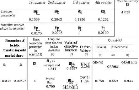
resulting point estimates are shown in Table 5.1. Only one constraint was binding at solution: its purpose was to ensure that the slopes involved in (3a) and (4a) were both close to unity. Details are shown in Table 5.2.

Table 5.1

Restricted Maximum Likelihood Estimates of the Double Logistic Model fitted in the First Differences under Hypothesis HA

Quarterly Data, 1980Q3–1993Q1

Parameters of displaced logistic for the saturation share of imports as a function of Australian competitiveness

1st quarter 2nd quarter 3rd quarter 4th quarter Price Sensitivity

γ

Location parameter

α

α

α

α

0.1069 0.2043 0.1186 0.1202

Minimum market

share for imports:

θ

θ

θ

θ

0.0175 0.0003 0 0.0100

Parameters of logistic trend in imports' market share Error correction parameter in eqn (3.11) Long- and short-run Arm-ington elasticities (a) Value of objective function (b) Durbin-Watson (c) Quasi-R2 ______________________________

(levels) (differences) ___________________________

(d) (e) (f)

a

b

ψ

σ_LRat sampleend 4.811

φ

QR2(W)

QR2(∆W)

QR2(∆ ln L)

18.039 -0.00525 0 typical_σ SR 0.790

[

φ

1.01 X 10

-3 ]

DW(4)

1.526 0.758 0.559 0.933

(a) σ

LR is calculated using (2.18); σSR is the sample mean of values calculated using (2.17). (b) φ_A is the residual sum of squares from the finally fitted equation (3.9).

(c) DW(1) and DW(4) are the 1st and 4th-order Durbin-Watson statistics; they refer to residuals from the fitted equation (3.9). Corresponding statistics for (3.10) are 0.972 and 1.554.

(d) QR2_{(W) is the square of the simple correlation coefficient between W}^

t and Wt. (e) QR2(∆W) is the square of the simple correlation coefficient between ∆W^_t and∆W_t.

(f) QR2_{(∆ ln L) is the square of the simple correlation coefficient between ∆ ln L}^ t and

∆ ln L_{t from fitted equation (3.19).}

Formula (2.18) indicates that when θ is small relative to K, the long-run substi-tution elasticity σ_LR is well approximated by the price sensitivity γ. Hence there is very little variation over time in the long-run substitution elasticity for the two quarters (namely, the second and third) in which imports' notional minimum share (at superlative levels of Australian competitiveness) is effectively zero in Table 5.1. The error correction parameter ψ is estimated to be zero to machine accuracy, thus favouring HA and the first-difference form (3.8) as the appropriate vehicle for

Table 5.2

Constraint Binding on Parameter Solution Presented in Table 5.1

Reference/

original form of Final value of

Final form of constraint/

[value of Lagrange constraint coefficient multiplier]

3(a) slope of sample

regres-sion of W on W^ = 1 1.00000

average over the 2 regressions of the absolute deviation from 1 of the regression slope ≤ 10-5

4(a) slope of sample

regres-sion of ∆W on ∆W^ = 1 1.00002 [-1.1103]

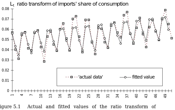
The error-correcting tendency of the model (which, with ψ = 0, lacks an explicit error-correction term) can be assessed (at least informally) from Figure 5.1, which shows the 'actual' values of L (i.e., the values computed from the realized values of the endogenous shares and from the fitted parameters) and the fitted values L^_t (computed from the exogenous variables and the fitted parameters). At least within sample, there seems to be little tendency for the fitted values to diverge from the 'observed' series as time progresses.

The seasonality of the data becomes very prominently displayed in the trans-form L. Figure 5.1 suggests that the parameterization on quarter-specific minimum shares θ and location parameters α successfully accounts for the seasonality. The estimates imply that only in the first and fourth quarters is imports' minimum possible ultimate share of consumption detectably above zero (θ_1(t) = 0.017; θ_4(t) = 0.010; or 1.7 and 1 per cent of the market respectively).

0 0.01 0.02 0.03 0.04 0.05 0.06 0.07 0.08

1 4 7 _{10 13 16 19 22 25 28 31 34 37 40 43 46 49}

'actual data' fitted value

Lt ratio transform of imports' share of consumption

Figure 5.1 Actual and fitted values of the ratio transform of imports' market share, 1980Q3−1993Q1

0.03 0.035 0.04 0.045 0.05 0.055 0.06 0.065

1 3 5 7 9 _{11 13 15 17 19 21 23 25 27 29 31 33 35 37 39 41 43 45 47 49 51}

actual import share

fitted import share (direct from levels)

Imports' market share of consumption

Figure 5.2 Projected and actual shares of imports in consumption, 1980Q3—1993Q1(estimated under HA)

Also of interest is the ability of the model to project changes in imports’ market share. The fitted and actual values of ∆W are shown in Figure 5.3.

-0.01 -0.005 0 0.005 0.01 0.015

0 5 10 15 20 25 30 35 40 45 50

actual changes in imports' share = W - W(-1)

fitted changes in imports' share [based on estimates in Table 5.1]

Figure 5.3 Projected and actual changes in shares of imports in consumption, 1980Q3—1993Q1(estimated under HA)

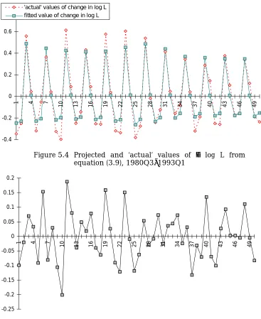
-0.4 -0.2 0 0.2 0.4 0.6 0.8

1 4 7

10 13 16 19 22 25 28 31 34 37 40 43 46 49

'actual' values of change in log L fitted value of change in log L

Figure 5.4 Projected and ‘actual’ values of ∆ log L from equation (3.9), 1980Q3−1993Q1

-0.25 -0.2 -0.15 -0.1 -0.05 0 0.05 0.1 0.15 0.2

1 4 7

10 13 16 19 22 25 28 31 34 37 40 43 46 49

Figure 5.5 Residuals from the fitted equation (3.9), 1980Q3−1993Q1

How confident can we be that the price responsiveness captured by our estimated γ is genuine? Formal tests of significance cannot be used for several reasons, including:

(I) The sampling properties of the estimator used here are unknown.

(2) The sample size (51) is very small relative to the number of parameters (12) estimated.

(3) The specification of the model was developed interactively with data exploration.

which minimizes the squared value of γ subject to the constraint set imposed in the earlier estimation.

In principle such a search could return the value 0 for γ. It seems that the nearest to 0 that γ can go without leaving the feasible set is 2.96 (versus 4.82 in Table 5.1).8 _{The lower role for substitutability in this parameter set results in a}

somewhat larger role for pure trend (b = -0.0065 versus -0.0053 in Table 5.1). Ignoring the constraint set and putting γ to zero, but keeping all other parameter values as in Table 5.1, causes the quasi-R2 for the level of imports’ market share to drop from 0.758 to 0.590; the fit for the differences actually improves from O.559 to 0.607.

When γ = 0, the model reduces to a (displaced) logistic time trend with quarter-specific upper and lower asymptotes. If constraints other than those for unbiasedness and those requiring the αs and θs to be non-negative are dropped, and φA is minimized subject to γ = 0, the model completely fails to track the dip

below trend in imports’ market share between quarters 22 and 32. This is shown in Figure 5.6. As shown in Figure 5.2, the results in Table 5.1 pick up this dip because of the coincident improvement in competitiveness (see Figures 1.2 and 6.2).

0.03 0.035 0.04 0.045 0.05 0.055 0.06 0.065

1 3 5 7 9 _{11 13 15 17 19 21 23 25 27 29 31 33 35 37 39 41 43 45 47 49 51}

actual import share

fitted import share (direct from levels)

Imports' market share of consumption

Figure 5.6 Fit of model, 1980Q3−1993Q1, when price influences are removed (i.e., γ = 0)

8 _{Here ‘feasible set’ excludes the DW restrictions, but includes the unbiasedness}

restrictions. The estimates of the parameters and fit statistics obtained are as follows: α^ = (0.1058, 0.2206, 0.1151; 0.1176); γ^ = 2.959; θ^ = (0.0176, 0.0003, 5.622×10-5

, 0.0010); a = 18.653; b = –0.00650;

σ

For the reasons listed above, we cannot put a confidence band around our estimate of b, the trend coefficient. We note, however, that the estimate of this parameter is relatively stable under the variations in estimation approach explored in this paper, consistently yielding values in the range -0.005 to -0.007. With competitiveness completely eliminated from the story, as in Figure 5.6, the estimated value of b is -0.00625.

Can we say anything about the cointegration (or lack thereof) of equation (3.9)? In a formal sense, no. However, without the need for error correction, there seems to be no tendency within sample for ∆ ln L and ∆ ln L^ to drift apart over time (Figure 5.4) ; the same is true of L and L^ (Figure 5.1). Perhaps more importantly, in the space of the primary data, W and W^ do not seem to be mutually diverging (Figure 5.2), nor do ∆W and ∆W^ (Figure 5.3).

5.2 Estimates under the moving-average hypothesis H_B?

It did not prove possible to satisfy simultaneously the unbiasedness criteria

(3a) and (4a) and obtain acceptable serial properties for the residuals from the levels equation (3.7). Results obtained with the unbiasedness restrictions, but not the DW restrictions, are virtually identical9 _{to those reported in Table 5.1, and are}

not reported here.

5.3 Interpretation of results, I — the bad news

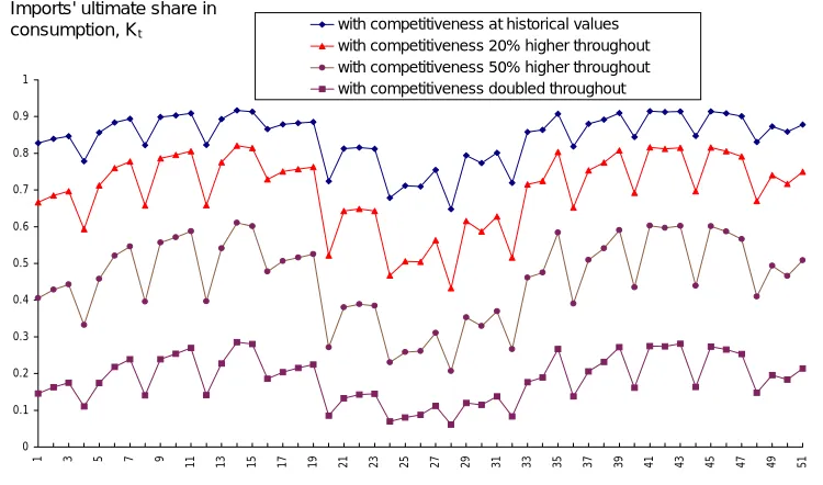
The bad news suggested by these results is that the ultimate penetration of the consumer goods market by imports is potentially very high: the values Kt of

imports’ ultimate market share at levels of competitiveness observed in the sample never fall below 71 percent in any of the estimates reported above. The time-series of the estimated within-sample values of K is shown in Figure 5.7.

0 0.1 0.2 0.3 0.4 0.5 0.6 0.7 0.8 0.9 1

1 3 5 7 9 _{11 13 15 17 19 21 23 25 27 29 31 33 35 37 39 41 43 45 47 49 51}

with competitiveness at historical values with competitiveness 20% higher throughout with competitiveness 50% higher throughout with competitiveness doubled throughout

Imports' ultimate share in consumption, Kt

Figure 5.7 Estimated values of imports’ ultimate share of con-sumption at levels of competitiveness that obtained during the sample, 1980Q3−1993Q1 (old data)

This news remains gloomy if one asks the question: by how much would competitiveness have had to increase in order to have lowered K by 30–40 percentage points throughout the sample period? This question roughly corresponds to the second lowest time path in Figure 5.7, which assumes that competitiveness throughout the sample were 50 percent higher than the historical values.

5.4 Interpretation of results, II — the good news

The above picture predicts a very substantial rise in imports’ ultimate share of the market even if Australian competitiveness were to reattain, and maintain, its highest sample value. The good news is that the trend coefficient b is relatively small. Using formula (2.11) we can deduce the approximate length of time which must elapse at a given level of competitiveness for the local product to lose (say) ten percentage points of market share:

(5.2) [dt]₁₀ = 0.1

{













K_t - W_t

K_t b Wt

}

.

At the end of the sample, this period is about 80 years if we work from Table 5.1, and slightly less if we use Table 5.3. Correcting for the linearization error inherent in (5.2) brings these values down to about 50 years. The displacement of the local product may be inexorable, but it is not rapid!

5.5 Interpretation of results, III — short-run price substitutability

Short-run elasticities of substitution vary over time at a fixed level of competi-tiveness because Wt on the far right-hand side of (2.17) does so. The estimated within-sample substitution elasticities σ_SR(t) are shown in Figure 5.7. The plot reveals wide variation from about 0.3 through about 1.8, with the highest values occurring at the historically highest levels of competitiveness.10

10 _{The reason for the positive relationship between σ}

SR(t) and competitiveness Pt can be

found by taking the total logarithmic differential of (2.17) and substituting for w_t from

(2.11). We find that, at fixed t, σ_SR(t) rises with K_t if and only if

{

( K_t - θ_t)(1 - K_t) +

W_t 1 - W_t

}

>

{

( K_t - θ_t)(1 - K_t) +

W_t

1 - W_t

}

0 0.2 0.4 0.6 0.8 1 1.2 1.4 1.6 1.8

1 4 7

10 13 16 19 22 25 28 31 34 37 40 43 46 49

sigma(SR) using Table 5.1

σ_SR(t)

Figure 5.8 Estimated values of short-run substitution elasticity between imported and domestically produced consum-ption goods, 1980Q3 through 1993Q1

6. New data release, revised estimates and post-sample tracking

The results reported in Section 5 used the data available in the middle of 1993 (when this study, conducted intermittently among other work, began). The above work was completed during the first quarter of 1996. By then new data were available. This presented an opportunity for post-sample evaluation of the model. Unfortunately, though, the more recent ABS data (national accounts and balance of payments data including the December quarter of 1995) have been rebased and come on a new set of definitions. Thus the post-sample data and the within-sample data are not readily compared.

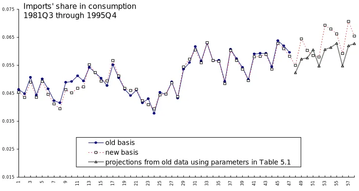
Data are available on both bases, however, from 1981Q3 through 1993Q1. This spans all but the initial four quarters of the sample which produced the results in Section 5. The data on imports’ share in consumption and on competitiveness on both bases is plotted in Figures 6.1 and 6.2 respectively.

0.015 0.025 0.035 0.045 0.055 0.065 0.075

1 3 5 7 9 _{11 13 15 17 19 21 23 25 27 29 31 33 35 37 39 41 43 45 47 49 51 53 55 57}

old basis new basis

projections from old data using param eters in Table 5.1

Im ports' share in consumption 1981Q3 through 1995Q 4

Figure 6.1 also shows the projections for the eleven quarters 1993Q2−1995Q4 obtained using the estimates in Table 5.1. Other than time, competitiveness is the exogenous variable driving the share projections. The latter are too low in ten out of the eleven quarters; part of the problem seems to be the different pattern of seasonality in the new data relative to the old — the seasonal peak in θ occurs in the September quarter in the new data, but in the March quarter in the old.

0 0.2 0.4 0.6 0.8 1 1.2 1.4

1 3 5 7 9

11 13 15 17 19 21 23 25 27 29 31 33 35 37 39 41 43 45 47 49 51 53 55 57 59

old basis new basis

Competitiveness 1981Q1 through 1995Q4

Figure 6.2 Data on competitiveness on old and new basis

Using the previously estimated parameter values as starting point, the model was re-estimated using the new data set. As before, it turned out that the restric-tions on the serial properties of the residuals and on unbiasedness could not be met simultaneously by these data. The restrictions on the Durbin-Watson statistics were dropped, yielding sample values of 2.37 and 1.33 at first and fourth order respectively.

One remaining constraint was binding at solution: namely, the one to keep the slopes of the regressions of W and ∆W on their respective fitted values close to unity (as in Table 5.2). The resultant estimates are shown in Table 6.1. Unfortunately, these are not the restricted MLEs; as we will see below, γ = 0 yields a higher value of the likelihood function. However, for reasons which will become clear presently, the estimates corresponding to the relative maximum reported in Table 6.1 are not without interest.

Fits of W in the levels and the differences are shown in Figures 6.3 and 6.4, while the fits of the differences of the log-ratio transform and the associated residuals are shown in Figures 6.5 and 6.6 respectively. All of these charts are based on Table 6.1.

Table 6.1

Estimates of the Double Logistic Model fitted in the First Differences under Hypothesis HA — Quarterly Data, 1981Q3–1995Q4*

Parameters of displaced logistic for the saturation share of imports as a function of Australian competitiveness

1st quarter 2nd quarter 3rd quarter 4th quarter Price Sensitivity

_γ

Location parameter

α

α

α

α

0.1540 0.2120 0.0838 0.1355

Minimum market

share for imports:

θ

θ

θ

θ

0 0.0096 0.0191 0.0003

Parameters of logistic trend in imports' market share Error correction parameter in eqn (3.11) Long- and short-run Arm-ington elasticities (a) Value of objective function (b) Durbin-Watson (c) Quasi-R2 ______________________________

(levels) (differences) ___________________________

(d) (e) (f)

a

b

ψ

σ

3.428

φ

0.3640

DW(1) 2.369

QR2(W)

QR2(∆W)

QR2(∆ ln L)

17.696 -0.00609 2.5×10−7 typical_σ SR 0.567

[

φ

1.178 X 10−3]

DW(4)

1.331 0.835 0.706 0.923

* These are not the restricted maximum likelihood estimates; see text.

(a) σ

LR is calculated using (2.18); σSR is the sample mean of values calculated using (2.17).

(b) φ_A is the residual sum of squares from the finally fitted equation (3.9).

(c) DW(1) and DW(4) are the 1st and 4th-order Durbin-Watson statistics; they refer to residuals from the fitted equation (3.9). Corresponding statistics for (3.10) are 0.708 and 1.604.

(d) QR2(W) is the square of the simple correlation coefficient between W^_{t and} W_t.

(e) QR2_{(∆W) is the square of the simple correlation coefficient between} ∆_W^

t and∆Wt. (f) QR2(∆ ln L) is the square of the simple correlation coefficient between ∆ ln L^_{t and}

∆ ln L_{t from fitted equation (3.19).}

0.03 0.035 0.04 0.045 0.05 0.055 0.06 0.065 0.07 0.075

1 3 5 7 9 11 13 15 17 19 21 23 25 27 29 31 33 35 37 39 41 43 45 47 49 51 53 55 57

actual import share fitted import share

,PSRUWV PDUNHW VKDUH RI FRQVXPSWLRQ

Figure 6.3 Projected and actual shares of imports in consump-tion, 1981Q3−1995Q4 (fitted values from Table 6.1 estimates)

-0.008 -0.006 -0.004 -0.002 0 0.002 0.004 0.006 0.008 0.01 0.012

-2 8 18 28 38 48 58

actual changes in imports' share

fitted changes in imports' share

Figure 6.4 Projected and actual changes in shares of imports in consumption, 1981Q3—1995Q4 (fitted values from Table 6.1 estimates)

-0.6 -0.4 -0.2 0 0.2 0.4 0.6 0.8

1 4 7 _{10 13 16 19 22 25 28 31 34 37 40 43 46 49}

'actual' values of change in log L fitted value of change in log L

Figure 6.5 Fit of logarithmic changes in the log-ratio transform, ∆ ln L, 1981Q3−1995Q4 (fitted values from Table 6.1 estimates)

-0.25 -0.2 -0.15 -0.1 -0.05 0 0.05 0.1 0.15 0.2 0.25

1 4 7 _{10 13 16 19 22 25 28 31 34 37 40 43 46 49}

Table 6.2

Estimates of the Double Logistic Model fitted in the First Differences under Hypothesis HA with Price Sensitivity set to Zero*

Quarterly Data, 1981Q3–1995Q4

Parameters of displaced logistic for the saturation share of imports as a function of Australian competitiveness

1st quarter 2nd quarter 3rd quarter 4th quarter Price Sensitivity

_γ

Location parameter

α

α

α

α

[by construction]

0.1605 0.2519 0.0775 0.1409

Minimum market

share for imports:

θ

θ

θ

θ

0** 0.0096 0.0182 0.0003

Parameters of logistic trend in imports' market share Error correction parameter in eqn (3.11) Long- and short-run Arm-ington elasticities (a) Value of objective function (b) Durbin-Watson (c) Quasi-R2 ______________________________

(levels) (differences) ___________________________

(d) (e) (f)

a

b

ψ

σ

0

φ

0.2841

DW(1) 2.02

QR2(W)

QR2(∆W)

QR2(∆ ln L)

19.465 -0.00713 2.5×10−7 typical _σ SR 0

[

φ

1.58 X 10−3]

DW(4)

1.690 0.763 0.759 0.924

* γ constrained to zero. To obtain the results reported here, the tolerances on the unbiasedness constraints had to be loosened somewhat, so that the intercept in the

regression of W_{t on} W^_{t = -0.001 and the associated regression slope is 0.9998.}

When the solution was recomputed with γ unconstrained, the algorithm found a solution indistinguishable from the one reported in the table above.

** Corner solution.

(a) σ

LR is calculated using (2.18); σSR is the sample mean of values calculated using (2.17).

(b) φ_Ais the residual sum of squares from the finally fitted equation (3.9).

(c) DW(1) and DW(4) are the 1st and 4th-order Durbin-Watson statistics; they refer to residuals from the fitted equation (3.9). Corresponding statistics for (3.10) are 0.392 and 1.621.

(d) QR2_{(W) is the square of the simple correlation coefficient between W}^

t and Wt. (e) QR2(∆W) is the square of the simple correlation coefficient between ∆W^_t and∆W_t.

(f) QR2_{(∆ ln L) is the square of the simple correlation coefficient between ∆ ln L}^ t and

0.03 0.035 0.04 0.045 0.05 0.055 0.06 0.065 0.07 0.075

1 3 5 7 9 11 13 15 17 19 21 23 25 27 29 31 33 35 37 39 41 43 45 47 49 51 53 55 57

actual import share fitted import share

,PSRUWV PDUNHW VKDUH RI FRQVXPSWLRQ

Figure 6.7 Projected and actual shares of imports in consumption, 1981Q3−1995Q4, when price influ-ences are removed (i.e., γ = 0) (estimated under HA).

This corresponds to the provisional restricted maximum likelihood estimates of the parameters.

Figure 6.2 reveals that most of the variation in relative prices took place towards the middle of the period spanned by the old data. The additional observations added by the new data include relatively little variation in competi-tiveness. Thus in the new data, accounting for seasonality and pure trend becomes relatively more important for obtaining a good fit and for maximizing likelihood. Consequently, trend and seasonal components alone give a good account in Figure 6.7 of the variation in imports’ market share, especially over the latter period of the sample. In terms of the likelihood, the failure to track the drop between quarters 18 and 28 is more than compensated for by the good fit obtained between quarters 36 and 58.

6.1 The bad and the good news revisited

In this subsection the estimates from Table 6.1 are taken as more plausible than those from Table 6.2. The strength of the trend against the local product according to the new data is somewhat stronger than that suggested by the old (b = -0.00609 versus -0.00525, according to Tables 6.1 and 5.1); but the effect of competitiveness in changing market shares is lower (γ = 3.4 versus 4.8).

0 0.1 0.2 0.3 0.4 0.5 0.6 0.7 0.8 0.9 1

1 3 5 7 9

11 13 15 17 19 21 23 25 27 29 31 33 35 37 39 41 43 45 47 49 51

with competitiveness at historical values with competitiveness 20% higher throughout with competitiveness 50% higher throughout with competitiveness doubled throughout

,PSRUWV XOWLPDWH VKDUH LQ FRQVXPSWLRQ .W

Figure 6.8 Estimated values of imports’ ultimate share of con-sumption at levels of competitiveness that obtained during the sample, 1981Q3−1995Q4 (new data, Table 6.1 estimates)

Likewise, the new data suggest a typical short-run elasticity of substitution that is a good deal lower than that suggested by the old data (0.57 versus 0.79 — see Tables 5.1 and 6.1). A loss in competitiveness therefore is projected to do less harm according to the picture projected by Table 6.1; on the other hand, the structural shift in favour of imports is stronger.

These ideas become firmer if we project the market share of imports in consumption using the parameter values of Tables 5.1 and 6.1. In Figures 6.9 and 6.10, market share is projected over the period 1996Q1 through 2042Q4. Three sets of assumptions are used:

• competitiveness remains as it was in 1995Q4

• competitiveness improves at 4 per cent per annum

• competitiveness deteriorates at 4 per cent per annum

(in Figure 6.9);







0 0.05 0.1 0.15 0.2 0.25

1 7

13 19 25 31 37 43 49 55 61 67 73 79 85 91 97 _{103 109 115 121 127 133 139 145 151 157 163 169 175 181 187 193 199 205 211 217 223 229 235 241 247 253}

projections from Table 6.2 projections from Table 6.1 projections from Table 5.1 actual data (old basis) actual data (new basis)

2042 Q4

1993 Q1

,PSRUWV VKDUH RI FRQVXPSWLRQ

2008 Q4

Figure 6.9 Projected trajectories of imports’ share in consumption according to estimated parameters shown in Tables 5.1, 6.1 and 6.2 when Australian competitiveness remains at its 1995Q4 value. The stronger trend in the new data is evident. With γ = 0, or with Pt fixed, the ceiling parameter K_t is subject to a stationary seasonal pattern (see eqn (2.4)); the gaps between the seasonal low and the seasonal high in the middle trajectory increase to almost 13 percentage points as t → ∞. This corresponds to a seaonal high of K equal to 0.929 and a seasonal low equal to 0.801.

0 0.05 0.1 0.15 0.2 0.25

1 8 _{15 22 29 36 43 50 57 64 71 78 85 92 99}

106 113 120 127 134 141 148 155 162 169 176 183 190 197 204 211 218 225 232 239 246 253

Imports' projected share with competitiveness decreasing by 4% p.a. from 1996 ownards [based on Table 6.1]

Imports' projected share with competitiveness decreasing by 4% per year from 1996 ownards [based on Table 5.1]

Imports' projected share with competitiveness increasing by 4% per year from 1996 ownards [based on Table 6.1]

Imports' projected share with competitiveness increasing by 4% per year from 1996 ownards [based on Table 5.1]

actual data (old basis)

actual data (new basis)

2042 Q4

2020 Q2

,PSRUWV VKDUH RI FRQVXPSWLRQ

2008 Q3 1993 Q1

Figure 6.10 Projected trajectories of imports’ share in consumption according to estimated parameters shown in Tables 5.1 and 6.1 when Australian competitiveness increases or deteriorates by 4 per cent per annum

explanation for the pattern of seasonal behaviour evident in Figure 6.9 is given in the caption to that figure.

Recall that the procedure of removing seasonality was developed in explor-ations with the old data. As we have seen above, the method works well within-sample for both data sets. Although the lowest curve in Figure 6.10 (which is based on coefficients estimated from the old data) does show a similar pattern of amplified seasonality during the middle part of the adjustment path, the effect is less pronounced. At all events, seasonality is a minor issue for the out-of-sample projections; if desired, a milder form of seasonality can be imposed on the annualized projections shown in Figure 6.9.

6.2 Summary of estimation results

Point estimates of the long-run elasticity of substitution between domestic and imported consumer goods are sensitive to the data set used — the (old) data terminating in the 1st quarter of 1993 yield a point estimate of 4.8, whereas

0 0.05 0.1 0.15 0.2 0.25

1 8

15 22 29 36 43 50 57 64 71 78 85 92 99 _{106 113 120 127 134 141 148 155 162 169 176 183 190 197 204 211 218 225 232 239 246}

imports' projected share with competitiveness decreasing by 4% per year from 1996 onwards [based on Table 6.1]

imports' projected share with competitiveness decreasing by 4% per year from 1996 onwards [based on Table 5.1]

imports' projected share with competitiveness increasing by 4% per year from 1996 onwards [based on Table 6.1]

imports' projected share with competitiveness increasing by 4% per year from 1996 onwards [based on Table 5.1]

2009Q1

,PSRUWV VKDUH RI FRQVXPSWLRQ

Figure 6.11 Projected trajectories of imports’ share in consum-ption according to estimated parameters shown in Tables 5.1 and 6.1 when Australian competitiveness increases or deteriorates by 4 per cent per annum, with seasonal variation removed in projection period

the rebased (new) data terminating in the 4th quarter of 1995 suggest a value of about 3.4, or alternatively, zero. Estimates of b corresponding to the old and the new data sets range between -0.005 and -0.007. These values for the pure trend parameter are relatively insensitive to variations in model specification (such as the elimination of the influence of prices) and to minor variations in data handling, suggesting that it may have a relatively tight sampling distribution.