Volume 16, Number 6 (November 1963)

IN THIS

ISSUE

A Method for the Characferisafion of Range-Type Vegetation

I. A. Nicholson and Roy Hughes 293 Converting from Brush to Grass Increases Wafer Yield in Southern

California____________________________ __ __ _...Lawrence W. Hill and Raymond M. Rice 300 Fertilization of Seeded Grasses on Mounfainous Rangelands in Northeastern

Utah and Southeastern Idaho..._________.._______~A. C. Hull, Jr. 306 Seed Yield of Russian Wild Ryegrass Grown on an Irrigated Clay Soil in

Southwestern Saskatchewan... . . . . ___ .____ ______________.____________.____ _____. ..T. Lawrence 311 Halogefon-Concern to Cafflemen..._AZZen D. Bruner and Jos. H. Robertson 312 The Effect of Intensify and Season of Use on fhe Vigor of Desert Range

Planfs..._.._..._~___________~~__~_~~_____C. Wayne Cook and L. A. Stoddart 315 Comments on Range Management Technical Assistance in the Middle East

with Special Refelrence fo Saudi Arabia...._...HaroZd F. Heady 317 Grazing in Relation to Runoff and Erosion on Some Chaparral Watersheds

of Central Arixona... Lowell R. Rich and Hudson G. Reynolds 322 The Grasslands of the Wesf... ________________________ Theodore A. Neubauer 327 Earthen Windbreaks, a New Management Device for Salt Marsh Rangelands

Thomas N. Shiflet 332 Spray Penetration in Scruboak with Helicopter Application

R. F. WagZe and CZive M. Countryman 333

Current Li~erafure..._____________._____..__._____.___.____.__.._._...__________________._.__~__._._. 335 News and Nofes... ____ _ _._________ _______________________ ________________________________________ __.__ ._____ _____ _.__________ 339

Wiih the Seciions... ________.__ _ ._____ _____________________________________________________________.______~ __________________ 342 Society Business... ____ ________________________________________.____~___.__________~________.___.__~._~__~ __________________.__ 346

Cover Photo - At Home for the Winter

Journal of

RANGE

MANAGEMENT

A Method for the Characterisation

of Range-Type Vegetation

I. A. NICI-IQLSON AND ROY HUGHES

Head of Agronomy Department, Hill Farming Research Organization, Edinburgh, Scotland and Agronomist, Welsh Plant Breeding Station, Aberystwyth, Wales, respectively. Mr. Hughes was formerly also with the H.F.R.O., Edinburgh.

In the last 30 years spectacular advances have been made in the production and use of pasture.

In particular, these develop-

ments have taken place on the better soils and in temperate cli- matic regions. In many parts of

the world today, however, in-

creasing attention is now being focussed on the more extensively used permanent grazings which are inherently unsuited to in-

tensive husbandry techniques.

Davies (1960) has recently dis-

cussed these grasslands and

classified them on a global basis into five categories according to their productivity. The two low- est categories, accounting for 68 percent of the total permanent grassland area of the world, he

describes as “extensive” and

“very extensive” carrying ten

“cattle units” and one to five such units per 100 acres, respec-’ tively. The cattle ranches of the western hemisphere, Africa and Australia, together with the up- land grazings of Western Europe,

come into the “extensive” pas-

toral group, while the “very ex- tensive” group includes those of

Patagonia, Northern Australia

and many types in Africa. Fun-

damentally, the problems of

these grazings are ecological and generally the management tech-

niques evolved in regions of

more intensive production can-

not be applied to them. Simi- larly, many of the well estab- lished techniques in pasture re- search are not appropriate for studies under extensive manage- ment regimes and special meth- ods are often needed.

In Great Britian, there are ap- proximately 14 million acres of upland “rough grazings” of low productivity used for livestock

production and this area com-

prises 29 percent of the available agricultural land. The vegetation

of this range land, within a

fenced or unfenced grazing unit of 300-1,000 or more acres, may exhibit a high degree of botani-

cal uniformity being composed

essentially of a single vegetation

type, e.g. a community domi-

nated by purple moor-grass (Mo-

Zinia caerulea (L.) Moench) ,

mat-grass (Nardus stricta

L.) ,

Bent/fescue species (Agrostis

L./Festuca L.) or heather (Cal-

Zuna vulgaris (L.) Hull). Much

more commonly, however, the

vegetation is distributed as a

mosaic of several different types or shows well defined altitudinal zonation. As the stocking rate is generally low, e.g. three to eight acres per sheep or 20 or more acres per cattle beast, large plots

293

are usually required in grazing studies. Where the vegetation

within the plot enclosure is

mixed, with pronounced spatial heterogeneity, it becomes diffi- cult to characterise the area and follow vegetation changes with- out adopting laborious and time-

consuming methods. The tech-

nique described in this paper was

developed for use under such

conditions.

Requirements of the Technique and ifs Use

The need for a suitable survey method arose with the establish- ment of a grazing experiment in

1950. This involved a simple

comparison of two contiguous

plots, each of approximately 40 acres, on deeply dissected ter- rain bearing a distinct vegeta- tional mosaic. Callunetum2 was the largest single community, but though heather was strongly dominant throughout its range, there were important changes in associated species with altitude.

An aerial photograph of the

--

1The authors wish to acknowledge the advice given on the statistical analysis by Dr. M. R. Sampjord of the Agricultural Research Council Unit of Statistics, Aberdeen and also for the assistance of Miss P. F. Ritches of the Hill Farming Re- search Organization. The authors are also indebted to the British Air Ministry for permission to publish the aerial photograph in Figure 1. 2The suffix -etum added to the gen-

294 NICHOLSON AND HUGHES

Yas .

SCALE

32

31

30

29

28

27

26

25

24

23

22

21

20

19

18

17

16

15

14

13

12

11

10

9

8

CHARACTERISATION OF RANGE-TYPE VEGETATION 295

area (Figure 1) gave useful in-

formation, but further data were

needed for its detailed interpre-

tation. The following require-

ments were considered necessary

in the design of a suitable tech-

nique.

1. Speed of operation in mak-

ing periodic measurements on

each plot or part of it.

2. Representation

of the

spatial distribution and extent of

the main communities and their

variants.

3. A sufficient measure of the

specific composition

of com-

munities to enable variation to

be detected where this was not

expressed in the character of the

dominant.

The requirements therefore

combined the essential features

of mapping with those of more

detailed vegetational analysis.

Methods of surveying

and

measuring vegetation have been

reviewed

by Brown. (1954).

Briefly, it can be said that con-

ventional techniques were not

readily applicable to the experi-

mental area or suitable for the

experimental

requirements

either because of their laborious

nature or, as in the case of recon-

naissance methods, b e c au s e of

their limitation in terms of ac-

curacy and detail.

Outline of the Method

The method finally developed

was based on point sampling us-

ing a two pronged fork3.

Since the boundaries of com-

munities were required, there

was little alternative

to sysi

tematic sampling if stations were

to be restricted to a manageable

number. The sampling stations

were therefore sited at regular

intervals along a series of equi-

distant transects. The plot taken

3The authors are indebted to Mr. P. J. Faulks, Senior Lecturer in Bot- any, University of Aberdeen, who advocated the use of a two-pronged fork for vegetational analysis and who made many valuable com- ments in the early stages of the work.

as an example

in this paper

measured 300 by 750 yards and

transects were laid out at right

angles to the long axis at 22-

yard intervals, measured hori-

zontally irrespective of s lop

There were 34 transects, most of

which were 300 yards long, the

sampling interval

along each

transect being three yards. The

area was thus divided

into

squares three by 33 yards with

samples taken at the grid inter-

sections. Sampling

with two

points at each station and re-

cording only the first species hit

by the descending needles (with

a distance of three inches be-

tween prongs) gave the mini-

mum number of points necessary

to provide some information on

species relationships

over the

mosaic. This procedure enabled

the data to be used for mathe-

matical characterisation of the

vegetation and also for the con-

struction of a “point” map to

show its distribution (Figure 1).

In the field, transects laid out

with a theodolite were perma-

nently marked at various points

according to the terrain.

The

three-yard sampling interval

was estimated by pacing after

previous practice under various

slope and other conditions. Al-

though the transects were ac-

curately positioned, the vertical

axes of the grid were thus only

estimated. As the errors in pac-

ing were different for each tran-

sect, the vertical axes therefore

departed from straight lines ac-

cording to the magnitude of the

errors on each transverse.

In

practice, as shown later, this did

not constitute a serious limita-

tion of the method.

Consfrucfbn of the Map

The outline of the map (Fig-

ure 1) is drawn to scale and the

transects shown as belts, stations

being represented by 99 pairs of

squares straddling

the center

line. Intervals between stations

are eliminated and the stations

are represented by a sequence

of contiguous squares in which

the appropriate species symbols

are drawn.

Statistical Treatment

In this paper, statistical work

is restricted to an examination

of the associations between each

of three selected species and all

other species. The main purpose

of this is to indicate, by applica-

tion of a chi-square test, how the

data can be used to give con-

siderably more information

about the vegetation than by the

use of frequency alone. (For an

account of a similar approach

using a more critical technique,

see Williams and Lambert {1959

and 1960) .)

In preparing the data for anal-

ysis contingency

tables were

constructed showing the class

frequencies

(number

of sta-

tions) of all relevant paired oc-

currences. Only class frequen-

cies with expected values of >5

were examined and the signifi-

cance level was fixed at P< .05.

Examination of the Method

Field Work

The most laborious part of the

work lay in marking out the par-

allel transects,

a procedure

which required one theodolite

operator and two assistants. The

time taken per transect varied

with topography and thus the

distance which could be ranged

from the theodolite

without

changing its position. On mod-

erately sloping ground, however,

any incompleted section of line

was easily continued by unaided

visual ranging with surveyor’s

poles. On the easiest terrain the

transects were marked out al-

most as rapidly as the position

of the theodolite

could be

changed. The sampling time for

a 300-yard-long transect varied

from about ten minutes

in

shrubby communities to about

thirty-five minutes where short

close-grazed turf predominated.

Accuracy in Delineating Plant Communifies

296

tograph (Figure 1) shows a

close similarity in the vegeta-

tional pattern as expressed by

the two methods. The main

zones of heather dominance for

example are clearly shown, to-

gether with the peripheral

It should also be noted

that in the aerial photograph the

top section of the plot is shown

in fairly uniform dark shades

(apart from the patchwork

caused by the burning pattern)

giving no indication of the spe-

cies associated with the domi-

nant. The map shows that a

variety of species are present in

this area and that the main

heather areas lack uniformity

both in the associated species

and in their frequency.

A series of measurements on

the photograph and on the map

have been used to estimate the

error in delineating community

boundaries along each transect.

Differences as low

as 0.3 per-

cent have been found where the

ground was fairly level, though

in one or two cases on very bro-

ken ground discrepancies as high

as 13 percent have been found4.

To mitigate the tendency for high

errors on undulating terrain it

is an advantage if several ver-

tical lines are laid down at right

angles to the transects to reduce

the cumulative pacing error.

Florisfic Composition and Species Relationships

The species recorded on the

map and the appropriate sym-

bols or index letters used are

shown in the list below.

As the first species hit by each

needle of the sampling fork is

the only one recorded there is a

tendency for the shorter or pros-

trate species to be underesti-

4It

successive

NICHOLSON AND HUGHES

mated. The most detailed infor-

mation on the composition of

the community

is therefore

given in short single-layered

types, but even in tall dense veg-

etation such as vigorous Callune-

turn or bracken stands, differ-

ences in community structure

are revealed except where the

upper canopy

is completely

closed. In many types of exten-

sive characterisation, however,

any lack of detail in this respect

may not be regarded as a serious

disadvantage, particularly

as

any further information con-

sidered necessary can

be ac-

quired by more detailed local

studies as and when required.

n

cv

T

E

0

L/I

G

P

R

W

IQ

&I

Z

cx

Ea

Ev

Je

I

Heather

(L.) Hull)

Mouse-eared

chickweed

(Cerastium vulgatum L.)

Marsh thistle (Cirsium

(L.) Stop.)

Crowberry

L.)

Bell-heather

Crossleaved heather

(E.

tetralix L.)

Heath bedstraw

Weigel)

Common tormentil

(L.) Rausch)

Sheep’s sorrel

L.)

White clover

L.)

Blaeberry

L.)

Cowberry

Speedwells

L.

sPP*)

Sedges (Carex L. spp.)

Common cotton-grass

Honck.)

Draw-moss

Soft rush (Juncus effusus

L.)

Heath rush (J.

L

N

m

un

Ao

AP

l?5%!

E!l

!%I

Hl

H

Lo

Pa

Pt

cl a

cl 8

q

Woodrush

DC.

SPP.)

Bog asphodel

(L.) Huds.)

Brown bent-grass

canina L.)

Common bent-grass

Sibth.)

Sweet vernal-grass

L.)

Early hair-grass

L.)

Wavy hair-grass

champsia flexuosa

(L.)

Trin.)

Sheep’s

fescue

L.)

Red fescue

L.)

Yorkshire fog (Holcus

L.)

HOZCUS

L. spp.

Perennial rye-grass

L.)

Annual meadow-grass

L.)

Rough-stalked

meadow-

grass

L.)

Bracken fern

(L.) Kuhn)

Misc. mosses

Bare ground

Although the use of a two-

pronged fork imposes some sta-

tistical restrictions, it is of inter-

est to ascertain whether the as-

sociations of species pairs re-

corded in this way can give use-

ful guidance on the classification

of communities with the area

as a whole.

CHARACTERISATION OF RANGE-TYPE VEGETATION 297

Table 1. Chi-square matrix for fransecfs 1-34 (whole plot area)

Heather 3 2 17 4* 2 0 1 9** 6* 35** 1 lO* 81** Bent grasses 13** 13** 0 lo** 24** 5* 7** 2 33** _ 120** _ _ 227**

Bracken 0 0 -8**1 --100 2 0- 12

Total 16** 15”” 1 25** 29”” 7 7” 4 42*” 6” 157”” 1 10”” 320*” (Values of chi-square not calculated for expected values < 5)

For column totals, chi-square= 6.0 (5%) = 9.2 (1%) For row totals, chi-square X15.5 (5%) =20.1 (1%) Degree of association of:

Heather with blaeberry’$

Bent grasses with misc. mosses,** fescue*!‘* and heath bedstraw * *

Bracken

Degree of association of:

Heather with fescues* *, HoZcus*, heath bedstraw** and misc. dicot species. * Bent grasses with bell heather**, wavy

hair-grass**, crowberrvzk” ” and blaeberry” *

Bracken with crowberry * *

ties” occur with a frequency less than the expectation. The bent- grasses are positively associated

with the fescues, mosses and

heath bedstraw and negatively

with bell heather, wavy hair- grass, crowberry and blaeberry. Bracken fern shows a positive association with no other species and is negatively associated with crowberry (one percent level). The main species groupings dem- onstrated by this analysis are thus:

a) heather/blaeberry b) bent/fescue grassland

The exclusion of the large

number of self: self occurrences from the analysis obscures the existence of large areas of rela- tively pure heather though in the case of bracken areas the ab- sence of significant associations with other plants indicates its

presence in relatively pure

stands.

More than Expected

Less The chi-square matrix for

than zone (1) is shown in Table 2. Expected _{Heather is positively associated}

The area was further ex-

amined by division into three zones, namely:

(1) Transects 1 - 9, character- ised by a predominance of gram-

inaceous communities, bracken

communities and zones of

heather dominance.

(2) Transects 10 - 20, consist- ing mainly of heather but also

containing small graminaceous

and bracken areas.

(3) Transects 21- 34, contain- ing mainly heather.

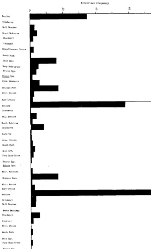
These zones can be picked out on the “point” map and specific

frequencies for each zone are

shown in Figure 2. Contingency tables were prepared for each

zone, but owing to the large

number of expected frequencies of < five in zones (2) and (3) and the high self: self occur- rences, especially of heather, a valid analysis of these zones was not possible.

only with wavy hair-grass,

which in this area has received

Table 2. Chi-square matrix for fransecfs 1-9

Heather 1 21”” - - 1 - 0 - 3 - 16** 0 3 45** Bent grasses 5” 19** - - 3 _ 0 - 4* - 15** - - 46** Bracken - 1 - - - 0 - 0 - - 1 Total 6* 41** _ _ 4 _ - - 7* - 31** - 3 92** (Values of chi-square not calculated for expected values < 5)

Degree of association of:

Heather with wavy hair-grass**

!

More Bent grasses with fescues* and heath bedstraw** than

Bracken Expected

Degree of association of:

Heather with heath bedstraw” * Bent grasses with bell heather* and

wavy hair-grass* * Bracken

FIGURE 2. Percentage frequency of species and groups of species in zones 1, 2 and 3.

a competitive advantage as a re- sult of burning and heavy graz- ing pressure. On suitable soils the succession from heather to bent/fescue grassland appears to have been completed as a result of these two factors, and the sep- aration of soils on this basis re- ceived added emphasis by the

highly significant negative as-

sociation (one percent level) of

heather with heath bedstraw,

one of the principal constituents

of bent/fescue grassland. The

bent-grasses are positively as- sociated with fescues and heath

bedstraw and negatively with

bell heather and wavy hair-

grass. Bracken shows no signifi- cant associations.

Floristic Change

The comparisons discussed

above are concerned with spatial

differences in vegetation at a

given time. Two areas of

strongly dominant heather, at

the north end of the area (be- tween transects 21 and 34)) were

burnt however after the first

analysis in 1956. The effect of

burning on the vegetation and

the subsequent nature of regen- eration is illustrated diagram- matically by construction of the “point” maps in Figure 3. Map

A shows the condition before

burning, Map B two years later and Map C eight years after burning.

Table 3 shows the percentage frequency of species for tran- sects 22 - 34 in the burnt and un- burnt areas for the three years 1954, 1958 and 1961. The general rise in frequency of heather in

the unburnt area reflects the

increasing dominance of the

plant. In 1958, two years after burning area B (the area was practically devoid of vegetation after the burn in 1956) consider-

able recolonisation had taken

place. Heather had greatly in- creased and bare ground was only 18 percent. Other species including wavy hair-grass were

Table 3. Florisfic changes in burnf and unburnt areas, 1954-61 (percent

frequency)

Unburnt Burnt

_

1954 1958 1961 1954 1958 1961

Heather 82.8 89.9 94.3

Blaeberry 5.1 0.9 0.7

Cowberry 1.6 0.6 0.3

Heath rush 1.1 0.9 0.4

Wavy hair-grass 1.0 0.6 0.2

Other species 7.1 6.0 4.0

Bare ground 1.3 1.1 0.1

- P -

100.0 100.0 100.0

83.7 55.3 74.4 5.6 9.1 7.1 2.0 3.7 2.4 2.2 4.5 3.5 0.4 4.1 3.3 5.4 5.3 6.0 0.7 18.0 3.3

- - -

CHARACTERISATION OF RANGE-TYPE VEGETATION 299

/ 24

23 22

FIGURE 3. “Point” maps of area covered by transects 22-34. Map A shows vegetation in 1954, Map R in 1958 two years after burning and Map C in 1961. Areas marked B on all maps indicate location of 1956 burn.

contributing noticeably to the

vegetation. By 1961 the succes- sion was considerably more ad- vanced with heather approach- ing its former prominent posi- tion. Other species were corres-

pondingly reduced though still

more prominent than before

burning.

Unfortunately the sampling

intensity was such that the data

available from the two small

burnt areas were considered to

be insufficient to allow a valid chi-square analysis to be carried out at the various successional

phases. The use of frequency

and preparation of a series of “point” maps for comparisons in

time, however, do demonstrate

the manner in which segments of the survey area can be iso- lated easily for more specific study without repetition of the entire survey.

Conclusions

The technique has been found to satisfy the requirements for

certain agronomic studies in

terms of speed and accuracy in the general characterisation of spatial pattern over an area, or on a given area at different times. It is simple and objective to operate and a map of con- siderable value can be produced readily. It is thought that the

method might be applicable to

a wide range of vegetation types, but from present evidence it is most suitable for use when the vegetation is disposed as a mo- saic of different communities, rather than where extensive uni- form areas occur. For many pur- poses, at least in preliminary work, it may be unnecessary to record individual species and in this case the use of a life form

characterisation may be ade-

quate, thus considerably reduc- ing the work.

The dimensions of the sam-

plinz fork i.e., the length of the prongs and their distances apart will depend on the nature of the vegetation, particularly regard-

ing its height and whether

closed or open communities are being studied. Although two in-

dependent points recorded at

each station would be statis-

tically more acceptable, experi- ence has shown that even this

departure from the technique

adds considerably to the sam-

pling time.

LITERATURE CITED

DAVIES, WILLIAM. 1960. Pastoral sys- tems in relation to world food supplies. The Advancement of Sci- ence, 17, 67, 272-280.

BROWN, DOROTHY. 1954. Methods of Surveying and Measuring Vegeta- tion. Commonwealth Bureau of Pastures and Field Crops Bulletin 42.

WILLIAMS, W. T. AND LAMBERT, J. M.

1959 and 1960. Multivariate Meth- ods in Plant Ecology.

I Association analysis in plant com- munities. Jour. of Ecol. 47: 83-101. II The use of an electronic digital computer for association analysis. Jour. of Ecol. 48: 689-710.

SpeciaMs

in

Qualify

N AT

1 V E G R A S S

E S

I

We grow, harvest, process these seeds Native Grasses Harvested in ten States _I Your Inquiries

Converting from Brush to Grass Increases

Water Yield in Southern California

LAWRENCE W. HILL AND RAYMOND M. RICE Research Foresters, Pacific Southwest Forest and Range Experiment Station, Forest Service, U. S. Department of AgricuZture, Glendora, California.

Southern California has no

monopoly on water supply prob- lems. But its problems are acute because of an unprecedented population increase accompanied by an overdraft of groundwater supplies. Most of California’s water comes from its wildland areas. In southern California,

brush-covered wildlands com-

prise about five and one half million acres. How these wild- lands are managed is one key to supplying some of the large and increasing demands for inexpen- sive and high quality water.

To help meet this challenge,

the San Dimas Experimental

Forest was established in 1933.2

A major objective was to de-

velop watershed management

methods that would produce

more usable water. This paper reports some answers we have found.

The Experimental Area

The 17,000-acre San Dimas Ex- perimental Forest stands on the southern slope of the San Gab- riel Mountains, about 35 miles east of Los Angeles. It is repre- sentative of the brush-covered mountains of southern Califor- nia. The land is highly dissected into numerous drainages which range from less than one square mile to more than 15 square miles. These are generally fan-

‘Presented at sixteenth annual meeting, American Society of Range Management, Rapid City, South Dakota, February 14, 1963. 2The San Dimas Experimental For-

est is maintained by the Forest Ser- vice in cooperation with the Cali- fornia Division of Forestry.

3CZimatic data are based on 27 years of record, 1933-l 960.

shaped and have short, steep stream channels and precipitous side slopes.

Rocks have been subjected to most of the recognized types of alteration, including folding and

faulting, extensive weathering

and erosion, extreme heat, and pressure. This geologic activity has resulted in the present com-

plex body of metamorphic and

igneous rocks. Because of fault- ing, the rock mass is extensively

and deeply fractured (Storey,

1947).

The soils on the Experimental Forest are generally residual and immature, moderate- to coarse-

textured, normally intermixed

with large amounts of fractured

rock, and very unstable. They

usually have no profile develop- ment, low water-retention capa-

city, and shallow depth. Only

seven percent of the area has soils greater than three feet deep

(Crawford, 1962).

A Mediterranean-type climate

prevails-dry, hot summers, and

rainy mild winters. Summer

temperatures often exceed

lOOoF., and winter temperatures seldom drop below 25”F.4 The

average annual temperature is

57.9”, and average annual evap-

oration (from free water sur-

face) is 64 inches. Annual pre- cipitation has ranged from 48.2

to 11.5 inches, averaging 26.7

inches. Nearly three-quarters of this falls from December through

March. Almost no rain occurs

during the summer.

Rainfall Disposition and Wafer Use By Plants

A rainfall disposition study on

an 875-acre watershed showed

that a considerable amount of

water was lost that might be

saved by alternative manage-

ment practice (Anonymous,

1955). Over a 15-year period the average loss from the watershed was more than 50 percent of the rainfall. The largest single loss was from evaporation (Table 1). If we could alter the kind,

structure, and density of the

watershed vegetation, we might r e d u c e evapotranspiration an d

increase streamflow. However,

many questions needed answer- ing before we finally selected

vegetation management as a

means for increasing w-ater

yield: What happens to precipi- tation once it reaches the soil? Do native plants differ in their

water requirements? _What

changes in vegetation do we

make, where, and how? If we

do get more water, what hap- pens to it? How much goes into

underground storage and how

much is realized as streamflow?

Lysimeter and plot studies

helped to answer some of these questions.

Lysimefer Study

Twenty-six lysimeters were

built in 1937 in order to compare water losses and yields under several kinds of plants native to the mountains of southern Cal- ifornia. Each lysimeter, a con- crete tank 10.5 feet wide, 21 feet long, six feet deep, was filled with uniformly-mixed soil. After a suitable calibration period pe- rennial grasses and native shrubs were planted in 20 tanks. Rain- fall, runoff, seepage, and soil moisture data were collected and analyzed for rainfall disposition differences between the several cover types (Patric, 1961; Sin- clair and Patric, 1959)

Compared to bare soil, vege-

tation markedly decreased run-

off (Table 2). Infiltration under grass and shrubs was more than twice that of the bare lysimeter during the low-rainfall period

and more than three times

greater during the high-rainfall period. Only under grass did ap-

CONVERSION INCREASES WATER YIELD 301

Table 1. Disposition of annual rainfall in Monroe Canyon, 1938-1939 fo 1952- 1953.

_____

15-year Driest year Wettest year average

Disposition 1950-1951 1940-1941 1938-1953

--- (Inches) - - - -

Rainfall 12 52 27

Interception 2 5 3

Evapotranspiration 10 14 12

_____-.-

Total Loss 12 19 15

Streamflow yield (l) 11 3

Groundwater yield (‘) 22 9

Total Yield (‘) 33 12

i Trace

preciable amounts of water perc- olate through the soil and be-

come available as net yield.

Since the grasses became dor- mant early in summer, they did not reduce soil moisture to the same extent and depth as did the deeper-rooted brush, which used water all summer. Conse- quently, less winter rainfall was needed to recharge the. grass- covered soil. The excess rainfall percolated below the root zone as water yield.

We can conclude from this

study that (a) plant cover in- creased infiltration, (b) perco- lation yields were always greater under the grass cover, (c) evap- orative losses under the grass did not differ markedly between low and high rainfall periods, and

(d) the study did not reveal how much water native plants might use in their natural environment.

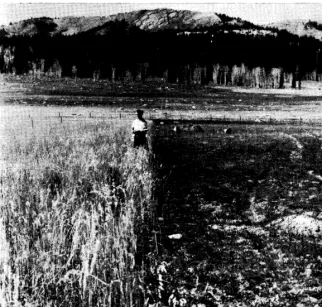
Plot Study

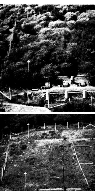
Before testing the lysimeter results on a watershed, a plot study was begun to find out if percolation yields could be in- creased by replacing deep-rooted brush with a shallow-rooted an- nual grass cover. This study was carried out under natural condi- tions (Figure 1).

For several years we measured rainfall, runoff, erosion, and soil moisture on nine hillside plots

heavily covered with native

brush, mostly scrub oak (Quer- cus dumosa). These plots had an average gradient of 35 per-

cent. The soil was a permeable, stony, sandy loam averaging 12 feet deep.

In 1951, we converted two sets (six plots) of plots to annual

ryegrass (Lolium multiflorum) ,

and left the third set undis-

turbed. During the next two

years we maintained a grass

cover on the converted plots by

killing all brush sprouts and

seedlings, and forbs with 2, 4, 5-T. The third year (1954-1955) we permitted a heavy stand of

summer-growing forbs to de-

velop.”

Once the grass cover was com- pletely established, no appreci- able amount of runoff or erosion

from the plots occurred. But the

change in vegetation greatly

altered water losses and soil

moisture relations (Rowe and

Reimann, 1961).

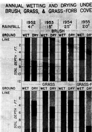
The soil of the undisturbed brush plots was wet to field ca- pacity through the la-foot depth the first winter. Rainfall that season totaled 41 inches. During the next three winters, however, rainfall was only 15, 25, and 20 inches, and the soil was wet to field capacity to depths of only four, nine and one half, and four feet. Each summer, evapotrans- piration dried the entire soil of these plots to near or below wilt-

ing point. Rainfall was not

enough after the first year to fully re-wet the soil (Figure 2). In contrast, the soil of plots

converted from brush to grass

was wet to field capacity the en- tire depth each rainy season. During the first three summers the grass-covered soils dried be- low field capacity to about seven feet and below wilting point to about three feet. Consequently, there was a greater carry-over of water in the three to la-foot depth of soil under grass than un- der brush at the end of summer.

A substantial soil moisture

Table 2. Annual rainfall disposition on the San Dimas lysimefers. average of five consecutive dry years and in one wef year.

.__

LOW RAINFALL PERIOD, 1952-1957

Evapora-

Surface Infiltration tive

Vegetation Rainfall runoff 1 Percolation loss2 --- (Inches) __-_---

Bare 20.6s 27.7 7.9 0 7.4

Brush4 20.6 3.0 17.6 0 17.6

Grass 20.6 3.4 17.2 1.8 15.7

HIGH RAINFALL PERIOD, 1957-1958

Bare 48.4 39.1 9.3 (5) 8.7

Brush4 48.4 19.4 29.0 3.8 24.6

Grass 48.4 20.3 28.1 11.5 16.5

-~

1 Not adjusted for interception. But, other studies have shown that brush intercepts about 11 percent of annual rainfall whereas grass intercepts about 6.5 percent.

2 Evaporative loss = rainfall - (runoff + percolation - increase or i- de- crease in soil moisture).

302 HILL AND RICE

FIGURE 1. Cover converted from brush to grass; before conversion, above; after con- version but before forbs were permitted to develop, below.

saving and potential ground-

water yield, 6.4 inches, was ob- tained under grass (Table 3) .

But when we permitted deep-

rooted, summer-growing forbs to invade the grass, soil moisture and percolation gains were lost

(Table 4). The soil throughout the 12-foot depth was nearly as dry by summer’s end as under the brush.

The study pointed out three important considerations. Vege-

tation conversion to increase

water yield (a) must be done on soils more than three feet deep, (b) the grass must be main- tained free of weeds, and (c) more than enough rainfall to re- place the soil water used by grass during the previous year must be received.

Managing For Increased Wafer Yield

Drawing on the results of the two earlier studies, we placed an

entire watershed under inten-

sive management to increase the

yield of usable water (Rowe,

1957).

Plants in the canyon bottom

have the most opportunity to

waste water. Consequently, for

our first water yield improve- ment trial, we removed 38 acres

of thirsty canyon-bottom trees

and brush from 875-acre Monroe

Canyon (Figure 3) during the

spring of 1958 and 1959. Volfe

Canyon, an adjacent 740-acre

watershed, was chosen as an un- treated control to evaluate treat-

ment effects in Monroe. These

drainages, similar in their hydro- logic and vegetal characteristics,

are comparable to many moun-

tain watersheds in southern Cali- f ornia.

4Forb.s included: common yellow mustard (Brassica campestris) , prickly lettuce (Lactuca serriola) , Douglas nightshade (Solanum douglasi), soap plant (Chlorogalum pomeridianum) , and Sierra thistle

(Cirsium californicum).

CONVERSION INCREASES WATER YIELD 303

FIGURE 2. Water-use differences under brush, grass, and grass-forb cover.

Chamise-chaparral and scrub

oak-chaparral formations, un-

burned since 1919, clothed the slopes.‘) Riparian woodland oc- cupied the canyon bottom and

covered about ten percent of

the watershed (87 acres). The

true riparian vegetation occu-

pied about ten percent of the area treated (3.8 acres). It con-

sisted of white alder (Alnus

rhombifolia), bigleaf maple (Acer macrophyllum), California laurel (Umbrellaria californica), willow (Salix spp.) , mulefat (Baccharis viminea), California

sycamore (Platanus racemosa),

and several associated herba-

ceous plants-about 25 acres of

the treated area were occupied by oak-woodland. The main spe- cies included California live oak (Quercus agrifolia), California

Table 3. Wafer regimen under brush and grass during a year of moderate rainfall, 1953-1954.

Water storage Evapo-

Vegetation Beg. of yr. End of yr. Rainfall Percolation transpira-

(10/19/53) (H/8/54) tion

--- (Inches) - - L - - - - -

Brush 9.9 11.4 24.9 0.0 23.4

Grass 21.6 24.9 24.9 6.4 15.5

laurel, interior live oak (Quercus wislizenii), bigleaf maple, can- yon live oak (Quercus chryso- Zepis), and bigcone Douglas-fir (Pseudotanga macrocarpa). Scat-

tered trees, native shrubs,

grasses, forbs, and rock outcrop occupied the remaining part of the cleared area.

Fifteen acres were cleared the first spring and 23 acres the next spring. The 1.3-mile long clear- ing varied from 100 feet to over 400 feet wide. It extended up the side slopes an average of 50 feet above the stream.

After clearing, the area was hand sprayed to kill sprouting

vegetation, brush seedings and

weeds. Native grasses, mostly

ripgut (Bromzbs rigidus), quickly invaded the area and provided good soil protection.

Treatment Effect on Waier Quantify

Water yield gains first ap-

peared during the summer and fall of 1958. With only 15 acres cleared, streamflow was 17.4 acre feet more than predicted with-

out treatment (Table 5). This

increase resulted from lower

day-to-day evapotranspiration

losses. Rainfall was light (1.8

inches) and contributed to

streamflow only the small

amount intercepted by the

stream.

304 HILL AND RICE

Table 4. Water regimen under brush and grass-forb cover during a year of moderate rainfall, 1955-1956.

Water storage Evapo-

Vegetation Beg. of yr. End of yr. Rainfall Percolation trans-

(1 l/9/55) (1 l/30/56) piration

Brugh Grass-forb

----w--e (Inches) - - - -

10.7 13.0 20.5 0.0 18.2

13.2 16.7 20.5 0.0 17.0

low the root zone of the previ- ously-cleared 15 acres. Here soil

moisture deficits were low so

that 8.4 acre feet of the season’s increased streamflow came from this area. The rest, 4.4 acre feet, resulted from lower day-to-day

evapotranspiration from all 38

acres cleared. This gain came

during inter-storm periods.

Streamflow gain the second

dry season, summer and fall,

1959, was 14 acre feet. Rainfall during the period was only 1.3 inches and contributed little to streamflow. As before, this sea-

son’s gain in streamflow was

principally due to lqwer day-to- day evapotranspiration.

During the second rainy season (winter and spring, 1959-1960) streamflow gain was eight acre- feet. Rainfall, 22.9 inches, was enough to satisfy soil moisture deficits. As in the 1958-1959 rainy season, the largest proportion of the gain came during and im- mediately after storms.

The largest gains in stream- flow came during the dry season when water is most needed. Be-

fore treatment, streamflow in

Monroe Canyon usually dried up in early July. Since the treat- men began, however, streamflow has been continuous.

Effects On Wafer Quality

Streamflow yields during the

rainy seasons were among the

highest on record (1934-1960)

yet no increase in storm dis charge or erosion rates was de- tected. In fact stream channel banks, and side slopes -some

of which eroded before treat-

ment-appeared to be complete-

ly stabilized. There were no

flood-producing storms during

cannot predict what effect clear- ing and subsequent grass cover establishment might have had on erosion and flood peaks.

Chemical analyses showed no trace of herbicides in the stream- flow. But small traces of oil (two

to 30 p.p.m.) used in the spray

mixture were found in some

samples.

Water temperature in Monroe Canyon appeared to be higher

than untreated Volfe Canyon.

During the summer, tempera-

tures were generally above 65°F. A relatively high concentration of green algae (Cladophora spp.) was associated with these tem- peratures.

The study was short-lived be- cause of a July 1960 fire. Never- theless, several conclusions can be drawn:

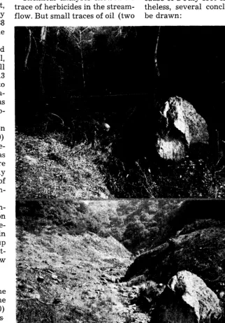
FIGURE 3. Part of the treated canyon bottom in Monroe Canyon; before clearing, above;

the same area after clearing, below.

CONVERSION INCREASES WATER YIELD

305

Table 5. Gains in sfreamflow from removing 38 acres of woodland-riparian vegeiafion in Monroe Canyon.

Rainfall Total gain Gain in Preceding During in streamflow per Season season season streamflow acre cleared

- - (Inches) - - --- (Acre feet) - - - First Year

Dry Seasoni 47.0 1.8 17.4 1.1

First Year

Rainy Season2 1.8 13.2 12.8 0.3

Second Year

Dry Season 13.2 1.3 14.0 0.4

Second Year

Rainy Season 1.3 22.9 8.0 0.2

First year total ____ 15.0 30.2 0.8 Second year total ____ 24.2 22.0 0.6 1 15 acres cleared

2 38 acres cleared

1. The study was conducted

during two years of below-aver-

age rainfall which were pre-

ceded by an above-average rain-

fall year. Gains in streamflow

during the post-treatment period

are probably associated with this

high rainfall as well as with the

treatment.

2. Seasonal gains in stream-

flow were less the second year

than in the first year. This de-

cline probably reflects the below

average rainfall conditions dur-

ing the second year’s rainy sea-

son. We would expect larger

gains with average rainfall.

3. Gains in streamflow were

highest during the dry season

when water is most needed and

lowest during the rainy season.

Streamflow has been continuous

since treatment began.

4. Dry season streamflow was

highest because the grass died

early in summer and, conse-

quently, used little soil water.

On the other hand, tree and

shrub growth in the control

watershed was in full foliage and

at the peak of annual growth. It

withdrew soil water all season,

and from a much greater depth.

5. If soils are not saturated

during the rainy season, treat-

ment may have little effect on

this season’s streamflow.

6. Streamflow gains were prob-

ably least from the area where

free water and wet soil surfaces

were exposed to wind and sun.

Gains were probably greatest

from the area where grass roots

did not penetrate continuously

saturated soil.

Multiple Benef ifs From Brush Conversion

We have demonstrated at San

Dimas that water yields can be

improved by converting canyon-

bottom vegetation from wood-

land-brush to a grass cover. At

present we are converting 140

acres of brush-covered

side

slopes with deep soil in Monroe

Canyon to grass cover. We ex-

pect additional yields in stream-

flow to result from this treat-

ment.

But water yield improve-

ments are not the only benefits

of a brush conversion program.

Extensive brush fields are bro-

ken into smaller, more manage-

able units for more effective fire

control. Grassed areas provide

for wildlife a new habitat that is

not found in dense brush. In

areas suitable for grazing, new

range for livestock is developed.

Research is underway at San

Dimas to determine the inte-

grated effect of some of these

multiple benefits.

LITERATURE CITED ANONYMOUS. 1955. Annual report.

U. S. Forest Serv., Calif. Forest 8~ Range Experiment Sta., 92 pp., illus.

CRAWFORD, JAMES M., JR. 1962. Soils of the San Dimas Experimental Forest. U. S. Forest Serv., Pacific Southwest For. & Range Exp. Sta., Misc. Paper 76, 20 pp, illus. PATRIC, J. H. 1961. The San Dimas

lysimeters. Jour. Soil 8~ Water Conserv. 16 (1) : 13-17.

ROWE, P. B. 1957. Plan for applied watershed management to in- crease water yield, Big Dalton Canyon, San Dimas Experimental Forest. U. S. Forest Serv. Pacific Southwest For. & Range Exp. Sta. 11 PP.

ROWE, P. B. AND REIMAN, L. F. 1961. Water use by brush, grass and grass forb vegetation. Jour. For- estry 59 (3) : 173-181.

SINCLAIR, J. D., AND PATRIC, J. H. 1959. The San Dimas disturbed soil lysimeters. Inter. Union Geodesy & Geophysics, Proc. 1959: 116-125.

STOREY, H. C. 1947. Geology of the San Gabriel Mountains, Califor- nia, and its relation to water dis- tribution. Calif. Dept. Nat. Re- sources, Div. Forestry, 19 pp.

Fertilization of Seeded Grasses on Mountainous

Rangelands in Northeastern Utah and

Southeastern Idaho1

A. C. HULL, JR.

Range Conservationist, Crops Research Division, Agri- cultural Research Service, U. S. Department of Agri-

culture, Logan, Utah

Fertilization has been widely

tested as a way to increase herb-

age production of western range-

lands. Eckert et

(1961) found

a response to nitrogen in the

eight to la-inch precipitation

zone in Nevada, but concluded

that fertilization would not be

practical. In North Dakota, with

17 inches of precipitation, Rogler

and Lorenz (1957) obtained an

average of 2,271 pounds of air-

dry herbage per acre per year

from a heavily grazed native

pasture when they applied 90

pounds of nitrogen per acre for

six successive years. Unfertilized

range yielded 748 pounds per

acre. Two years of fertilization

did more to improve the range

than six years of complete iso-

lation from grazing.

On Colorado’s Front Range

McGinnies (1962) worked on

five sites with precipitation of

12 to 16 inches. He found that

nitrogen increased

herbage

yields on older seeded grass

stands on average or better sites

and in years of average or above-

average precipitation.

Eckert

and Bleak (1960) determined

that four mountain soils with 15

to 40 inches annual precipitation

in western Nevada and northern

1 Cooperative investigations of Crops Research Division, Agricultural Re- search Service and the U. S. Forest Service, U. S. Department of Agri- culture; and Utah Agricultural Ex- periment Station, Logan, Utah. Thanks to Wesley Bitters and Steven Smith, former students who assisted with the study and to Dr. R. L. Smith for help on analysis of soil-nitrogen losses. Utah Agric. Expt. Sta. Journal Paper 316.

California were deficient in ni-

trogen, phosphorus, and lime.

Retzer (1954) obtained no im-

portant increase in native herb-

age by top dressing with 14 fer-

tilizers and minor elements on

seven range soils on sites with 15

to 30 inches of precipitation in

the Rocky Mountains.

Gomm (1962) worked in a

high-altitude park in Montana,

where the annual precipitation

was 25 inches. He found that fer-

tilizers probably decreased the

number of established seedlings.

Hull et

(1962) applied several

fertilizers spring and fall for

three years on new range seed-

ings on six mountainous areas in

the West where precipitation

ranged from 12 to 40 inches an-

nually. They found that nitro-

gen increased seedling numbers

at one location and increased

vigor of seeded and native plants

at most locations.

On many dry ranges where

moisture limits plant growth

and on some mountainous areas

where precipitation is high, fer-

tilization has given erratic re-

sults. The present studies were

initiated to test the response of

seeded grasses on mountainous

rangelands to commercial ferti-

lizers.

FIGURE 1. General view of the Logan Canyon area where fertilizers were applied in 1957 and 1958.

Experimental Procedures and Resulfs

This paper

reports

three

studies separately: (1) Fertiliza-

tion of pubescent wheatgrass

(Agropyron trichophorum

(Link) Richt.) in northeastern

Utah, (2) Fertilization of new

seedings in southeastern Idaho,

and (3) Fertilization of a mix-

ture in southeastern Idaho.

Nitrogen (N) was appplied as

ammonium nitrate and phos-

phorus (available P,O,) as treble

superphosphate on the soil sur-

face. Results were measured by

numbers of plants per square

foot or by pounds of air-dry

herbage per acre. Chemical con-

tent of the herbage was deter-

mined in the third study. Soil

and herbage samples were ana-

lyzed by standard procedures.

Significance of results at the

five-percent

level was deter-

mined by Duncan’s (1955) mul-

tiple range test.

Ferfilizafion of Pubescent Wheafgrass in Northeastern Ufah

The experimental area was a

big sagebrush

Nutt.) covered opening in

the spruce (Picea spp.) and fir

(Abies

spp.) zone at an elevation

of 7,700 feet in Logan Canyon

(Figure 1). Aspect was south-

west with a 15-percent slope.

Nearby snow survey and summer

precipitation records showed an

annual precipitation of approxi-

mately 32 inches; 4.5 inches of

rain June to September and 27.5

inches of late fall rain and win-

ter snow. Snow usually covered’

the area from mid-November to

mid-May. The soil was a loam

Soil characteristics at the zero to

six and six to 12-inch depths be-

fore treatment were as follows

(data for the shallow depth are

listed first): pH (saturated

paste) 6.3, 6.5; percent soluble

salts 0.02, 0.02; organic matter

percent 6.9, 4.1, nitrogen percent

0.3,0.2; and pounds P,05 per acre

390, 241.

Pubescent wheatgrass

was

seeded in the fall of 1953. A good

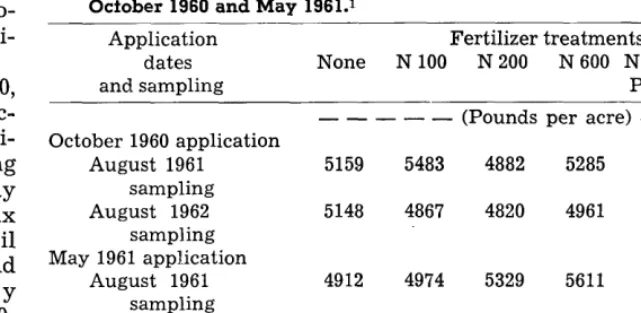
FERTILIZATION OF GRASSES

stand of grass resulted. Three

replicates of six fertilizer treat-

ments listed below were applied

to one series of plots in October

1957 and to another series in

June 1958.

Results:

Rates of fertilizer

(pounds per acre) applied both

spring and fall and average air-

dry grass production (pounds

per acre) in 1958 were: No fertil-

izer, 760; N 20, 685; N 40, 718;

N 60, 842; N 40 and

791; and P,O, 200, 811. Although

fertilizers were associated with

increased grass yields, the differ-

ences were not significant. There

was no significant difference

between spring and fall applica-

tion. Favorable moisture in 1959

caused yields which were almost

double those in 1958, but again

there was no significant differ-

ence in grass growth or yield.

There were no visible differ-

ences either year in season of

growth, color, or vigor of the

grass as the result of fertilizer

treatments.

Feriilization of New Seedings in Soufheasfern Idaho

The study area was a weedy

opening at 8400 feet elevation in

the spruce-fir type in Franklin

Basin, southeastern Idaho. The

aspect was west with a three-

percent slope. Snow normally

covered the area from late Octo-

ber to June 1. Five-year snow

survey and summer precipitation

records averaged 42.3 inches an-

nually. Winter snow and late-

fall rain amounted to 36.2 inches;

rain from June to September 6.1

307

inches. The first 12 inches of soil

were a silt loam with clay loam

below. Calcium carbonate at all

depths was 0.2 percent (Table 1).

Ten seeding methods were

used in the fall and three in the

spring with four replications for

three years (1957-1960). The fol-

lowing species were seeded sep-

arately in each seeding method;

intermediate wheatgrass

pyron intermedium

(Host)

Beauv.) ,

slender wheatgrass

(Link)

pu-

bescent wheatgrass,

smooth

brome

Leyss.) ,

and hard fescue

var. duriusculu (L.) Koch).

Five fertilizer treatments were

applied at right angles to all

seeded rows at the following

pounds per acre at the time of

seeding: (1) No fertilizer; (2)

N 100; (3) P,05 200; (4) N 100

and P,O, 200; and (5) N 100, P,O,

200, potash (K,O) 100, sulfur (S)

100, copper sulfate 50, ferrous

sulfate 50, magnesium sulfate 50,

manganous sulfate 50, zinc sul-

fate 50, sodium borate 20, and

ammonium molybdate one pound

per acre.

Seedlings were counted spring

and fall for three years after

seeding. Notes were made on

height and vigor of seeded and

native species.

Results:

Averaging all five spe-

cies on all seeding treatments

gave the following plants per

square foot for the five fertilizer

treatments listed above: 0.8, 0.7,

0.7, 0.6,0.6. Fertilizer application

did not significantly affect plant

Table 1. Soil characferisfics at Franklin Basin before fertilizers were ap- plied.

Moisture percent

Soil Potas- Organic Satura-

depth PH Salts sium P205 N matter 15 Y3 tion

(Satu-

rated (EC x (me/100

(Inches) paste) 103) g.) (WA) (Percent) (Atmospheres)

o-3 5.9 .26 1.04 66 .20 3.9 11 29 45

3-6 5.9 -22 .72 49 .20 3.8 11 28 48

6-12 5.7 .18 .62 - .15 3.0 12 27 47

12-24 5.6 .21 .58 - .ll 2.0 12 26 44