MPC Based Fuzzy Logic Controller for Non
Linear Process
Rajesh.T
1 ,Dr.G.M.Tamilselvan
2, Arun jayakar.S
3Assistant Professor, Dept. of EIE, BannariAmman Institute of Technology, Sathyamangalam, Erode, India1
Pprofessor, Dept. of EIE, BannariAmman Institute of Technology, Sathyamangalam, Erode, India2
Assistant Professor, Dept. of EIE, BannariAmman Institute of Technology, Sathyamangalam, Erode, India3
ABSTRACT: Non linear process is the immense challenge in process control and it cannot be effectively controlled by means of conventional linear P+I+D controller. Hence an attempt is made in this paper as Model Predictive Control algorithm based fuzzy logic controller design for conical tank level control. For each stable operating point, a first order process model was identified using process reaction curve method. The real time implementation is done in simulink using MATLAB. The experimental results shows that proposed control scheme have good set point tracking and disturbance rejection capability.
KEYWORDS: MPC;PID;Fuzzy;Conical tank;MATLAB
I. INTRODUCTION
In most of the process industries controlling of level, flow, temperature and pressure is a challenging one. Based on the plant dynamics, they may be classified as linear and non-linear processes. In level control process, the tank systems like cylindrical, cubical are a linear one, but that type of tanks does not provides a complete drainage. For complete drainage of fluids, a conical bottomed cylindrical tank is used in some of the process industries, where its nonlinearity might be at the bottom only. The drainage efficiency can be improved further if the tank is fully conical. But continuous variation in the tank system makes it highly non-linear and hence the liquid level control in such systems is difficult. A conical shaped tank system are mainly used in Colloidal mills, Leaching extractions in pharmaceutical and chemical industries, food processing industries, Petroleum industries, Molasses, Liquid feed and Liquid fertilizer storage, Chemical holding & mix tank, Biodiesel processing and reactor tank. To avoid settlement and sludge in Storage and holding tanks, the conical tanks are used.
II. PROPOSED WORK
A. EXPERIMENTAL SETUP
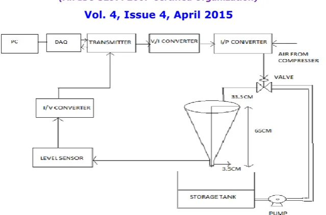
Figure 1: Level Control of Conical Tank System
Figure 1 shows the experimental setup of conical tank level control process
B. DESCRIPTION OF THE CONICAL – TANK LEVEL PROCESS
The tank is made up of stainless steel body and is mounted over a stand vertically. Water enters the tank from the top and leaves the bottom to the storage tank. The System specifications of the tank are as follows,
TABLE I
SPECIFICATIONS OF PROPOSED SYSTEM EQUIPMENTS DETAILS
Conical tank Stainless steel body, height– 65 cm, Top diameter–33.5 cm Bottom diameter – 3.5 cm
Differential Pressure Level Transmitter
Differential Pressure Level Transmitter
Pump Centrifugal 0.5 HP
Control Valve Size ¼ Pneumatic actuated Type: Air to open,
Input 3-15PSI
Rota meter Range 0-460 LPH
C. MATHEMATICAL MODELING OF PROCESS
A mathematical model is a description of a system using mathematical concepts and language. The process of developing a mathematical model is termed as mathematical modeling. Generally modeling of linear systems involves direct derivations whereas non- linear systems require certain approximations to arrive at the solution.
Types of Non-linear Approximations: Taylor Series Approximation
Optimal Approximation
Global Approximation
Jacobian Method
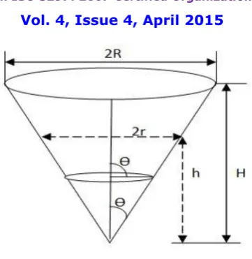
Figure 2: Mathematical Modeling Where,
R = Top radius of the tank H = Total height of the tank r = Radius at the liquid level (h) h = Level of the liquid (Variable)
tanƏ= r/h and also tanƏ=R/H (1)
Therefore, r/h=R/H (2)
R =(R*h)/H (3)
Area A=πr2 (4)
dA/dt=d{π((R*h)/H)2}/dt (5)
=π(R/H)2 *2h dh/dt (6)
Volume V=1/3 *πr2 h (7)
=1/3*Ah (8)
dV/dt=1/3*{A dh/dt+hdA/dt} (9)
=1/3 *dh/dt{A+2π(R/H)2*h2} (10)
By Newton’s law Fin-Fout=1/3 *dh/dt{A+2π(R/H)2*h2} (11)
Output flow rate, Fout= K ℎ (12)
Fin-𝐾 ℎ =1/3 *dh/dt{A+2π(R/H)2*h2} (13)
dh/dt = {3(Fin-𝐾 ℎ)}/{ A+2π(R/H)2*h2} (14)
dh/dt = {3(Fin-𝐾 ℎ)}/{ 3π(R/H)2*h2} (15)
= {(Fin-𝐾 ℎ)}/{ π(R/H)2*h2} (16)
α = 1/ π(R/H)2 (17)
β = Kα (18)
By Taylor’s series:
F(h,Fi) = f(hs ,Fis) + ( ∂f/∂h)(hs,Fis) (h-hs) + (∂f/∂Fi)(hs-fis)F(fi-Fis)
(20)
F(h,Fi) = f(hs ,Fis) - 2Fis hs-3(h-hs) + hs-2(F-Fis) (21)
h-3/ 2= hs -3/2
- (3/2)hs -5/2
(h-hs) (22)
dh/dt = α[ f(hs ,Fis) - 2Fis hs-3(h-hs) + hs-2(F-Fis)] - β[hs-3/2- (3/2)hs-5/2(h-hs)] (23)
At steady state,
dhs/dt = αFishs-2-βhs-3/2= 0 (24)
d(h-hs)/dt= -2αFishs-3(h-hs) + αhs-2(F-Fis)] + 3/2βhs-5/2(h-hs) (25)
dy/dt = -2αFishs-3Y + αhs-2U + (3/2)βhs-5/2Y (26)
dy/dt = -2βhs-3/2hs-1 y + αhs-2U + (3/2)βhs-5/2Y
= -(1/2) βhs-5/2y + αhs-2U (27)
(2/β) hs 5/2
(dy/dt) = -y + αhs-2U
τ(dy/dt) + y = (2α/β) hs1/2U (28)
τ(dy/dt) + y = CU (29)
Taking Laplace Transform,
Y(s)/U(s) = C/[τs+1] (30)
Where,
C = (2α/β) hs1/2Steady State Gain.
τ = (2/β) hs5/2Time Constant.
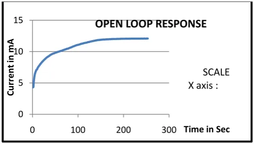
D. RESPONSE OF OPEN LOOP TEST:
The response of the open loop test as described in chapter 6.1 is given below. It shows that the steady state gain is 12mA and time constant 7.62 sec with input step change of 100LPH.
Figure 3: Openloop Response Cruve The obtained response from open loop test which represents
First order transfer function with zero dead time.
𝑮 𝑺 =𝑲𝒑𝒆−𝝉𝒅 (𝒔)
𝝉𝒔+𝟏 (31)
0 5 10 15
0 100 200 300
Cu rr e n t in m A
Time in Sec
OPEN LOOP RESPONSE
E. Linearization
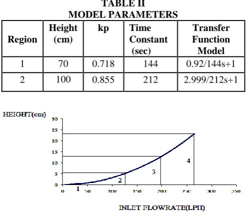
The process steady state input output characteristics thus obtained shows the non-linear behavior as the area varies in a non-linear fashion with the process variable height (h).To obtain a linear model process steady state input –output characteristics curve is divided into five different linear regions as shown in the fig 4
TABLE II MODEL PARAMETERS
Region
Height (cm)
kp Time Constant
(sec)
Transfer Function Model
1 70 0.718 144 0.92/144s+1
2 100 0.855 212 2.999/212s+1
Figure 4: Piecewise Linearization Curve
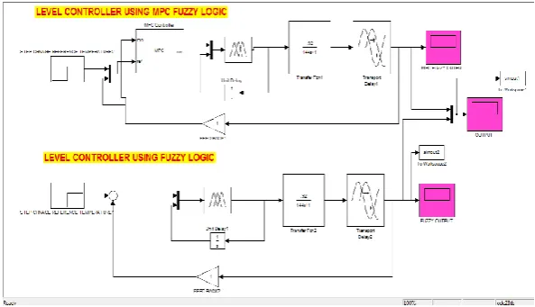
III. MPC BASED FUZZY CONTROLLER
MPC is a form of control in which the current control action is obtained by solving on-line. At each sampling instant, a finite horizon open-loop optimal control problem, using the current state of the plant as the initial state. The Optimization yields an optimal control sequence and the first control in this sequence is applied to the plant.
Figure 6: Concept of MPC
(32)
Equation 32 shows that step response model where Si = the i-th step response coefficient N = an integer
(the model horizon) y0 = initial value at k=0 Figure 6 shows that Model Predictive Control (MPC) – regulatory
controls that use an explicit dynamic model of the response of process variables to changes in manipulated variables to calculate control “moves”.
Figure 7:Fuzzy Rules
IV SIMULATION AND RESULTS
The simulation result of MPC based Fuzzy with various operating points was obtained using MATLAB environment. The performance of the proposed controller is compared with existing conventional controller.
This structures for compensate the disturbance model uncertainty. The procedure is focused on set point responses. But a good set point response denotes good disturbance rejection particularly for the disturbance occurs at the process input. The modified of the design procedure is developed to improve input disturbance rejection.
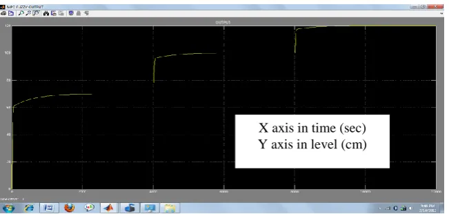
Figure 9: Simulation for Fuzzy output
Figure 10: Simulation for MPC based Fuzzy output
Figure 9,10 shows that the MPC based fuzzy logic controller having good set point tracking capability when compared to Fuzzy logic controller also the time domain specifications has to be normalized.
TABLE III
COMPARISION OF FUZZY AND MPC BASED FUZZY
Set point (Step input)
Controller Rise time (secs)
Settling time (sec)
70 Fuzzy 200 1100
MPC based Fuzzy
100 990
100 Fuzzy 420 4200
MPC based Fuzzy
310 3100
X axis in time (sec) Y axis in level (cm)
V. CONCLUSION
For practical applications or an actual process in industries MPC based fuzzy controller algorithm is simple and robust to handle the model inaccuracies and hence using MPC-Fuzzy tuning method a clear trade-off between closed-loop performance and robustness to model inaccuracies is achieved with tuning parameter. It also provides a good solution to the process with significant time delays which is actually the case with working in real time environment. As far as the tuning of the controller is concerned we have optimum control and prediction vector which compromises the effects of discrepancies entering into the system to achieve the best performance. Thus, what we mean by the best control horizon that gives the best MPC performance for the optimum Prediction value. Also the standard MPC based Fuzzy controller results in good set point response performances. The simulation results shows the MPC based Fuzzy controller have minimum settling time and rise time in order to reach steady state value when compare to conventional controller.
REFERENCES
[1] Mehta, S. ; Shah, P. ; Vaidya, V. Design and comparative study of PID controller tuning method from IMC tuned 2-DOF pole placement parameter structure for the DC motor speed control application Engineering (NUiCONE), 2013
[2] Hajare, V.D. ; Patre, B.M. Design of PID controller based on reduced order model and Characteristic Ratio Assignment method Control Applications (CCA), 2013 IEEE International Conference on Digital Object Identifier:
[3]Ananth, D.V.N. ; Kumar, G.V. ; Sobhan, P.V.S. ; Rao, P.N. ; Raju, N.G.S. Improved internal model controller design to control speed and torque surges for wind turbine driven permanent magnet synchronous generator Microelectronics and Electronics (Prime Asia), 2013 IEEE Asia Pacific
Conference on Postgraduate Research in
Digital Object Identifier:
[4]Venkatesan, N. Anantharaman, N.Controller design based on Model Predictive Control for a nonlinear process Mechatronics and its Applications (ISMA), 2012 8th International Symposium on Digital Object Identifier:
[5] Warier, S.R. ; Venkatesh, S.Design of controllers based on MPC for a conical tank system Advances in Engineering, Science and Management (ICAESM), 2012 International Conference on Publication Year: 2012 ,
[6] Sukanya R. Warier, SivanandamVenkatesh “DESIGN OF CONTROLLER BASED ON MPC FOR A CONICAL TANK SYSTEM”IEEE International Conference on Advances In Engineering, Science and Management (ICAESM - 2012) March 30, 31, 2012.
[7]Korkmaz, M. Aydogdu, O. Dogan, H.Design and performance comparison of variable parameter nonlinear PID controller and genetic algorithm based PID controller Innovations in Intelligent Systems and Applications (INISTA), 2012 International Symposium on Digital Object Identifier: [8] Anand, S. ; Aswin, V. ; Kumar, S.R.Simple tuned adaptive PI controller for conical tank process Recent Advancements in Electrical, Electronics and Control Engineering (ICONRAEeCE), 2011 International Conference on Digital Object Identifier: IEEE Conference Publications
[9] S.Nithya, N.Sivakumaran, T.K.Radhakrishnan and N.Anantharaman” Soft Computing Based Controllers Implementation for Non-linear Process in Real Time” Proceedings of the World Congress on Engineering and Computer Science(WCECS )2010,Vol – 2.
[10] N.S. Bhuvaneswari , G. Uma , T.R. Rangaswamy,"Adaptive and optimal control of a non-linear process using Intelligent controllers," Applied SoftComputing 9 , 182-190
[11] V.R.Ravi, T.Thyagarajan, M.MonikaDarshini“A Multiple Model Adaptive Control Strategy for Model Predictive controller for Interacting Non
Linear Systems”International Conference on Process Automation, Control and Computing (PACC),July 2011.pp:1 – 8.
[12] Qin S.J., Badgwell T.A., A survey of industrial model predictive control technology Control Engineering Practice, Vol.11, pp.733-746, 2003.
BIOGRAPHY
T.Rajesh was born in Virudhunagar, Virudhunagar District, Tamilnadu, India. He got his B.E degree (Electronics and Instrumentation Engineering) in Noorul Islam College of Engineering Anna University, Chennai, Tamil Nadu, India, In 2010 and received his M.E Control and instrumentation Engineering) in Anna University of Technology, Coimbatore, Tamil Nadu, India, In 2012. Now, he is working as Assistant Professor in Banari Amman Institute of Technology, Sathy, Tamil Nadu, India. He published many papers in various national and international journals, conferences. His research interests include in Control system and process control.