R E S E A R C H
Open Access
Accurate state estimation from uncertain data
and models: an application of data assimilation
to mathematical models of human brain tumors
Eric J Kostelich
1*, Yang Kuang
1, Joshua M McDaniel
1, Nina Z Moore
2, Nikolay L Martirosyan
2and Mark C Preul
2Abstract
Background:Data assimilation refers to methods for updating the state vector (initial condition) of a complex spatiotemporal model (such as a numerical weather model) by combining new observations with one or more prior forecasts. We consider the potential feasibility of this approach for making short-term (60-day) forecasts of the growth and spread of a malignant brain cancer (glioblastoma multiforme) in individual patient cases, where the observations are synthetic magnetic resonance images of a hypothetical tumor.
Results:We apply a modern state estimation algorithm (the Local Ensemble Transform Kalman Filter), previously developed for numerical weather prediction, to two different mathematical models of glioblastoma, taking into account likely errors in model parameters and measurement uncertainties in magnetic resonance imaging. The filter can accurately shadow the growth of a representative synthetic tumor for 360 days (six 60-day forecast/ update cycles) in the presence of a moderate degree of systematic model error and measurement noise. Conclusions:The mathematical methodology described here may prove useful for other modeling efforts in biology and oncology. An accurate forecast system for glioblastoma may prove useful in clinical settings for treatment planning and patient counseling.
Reviewers:This article was reviewed by Anthony Almudevar, Tomas Radivoyevitch, and Kristin Swanson (nominated by Georg Luebeck).
Keywords:State estimation, data assimiliation, mathematical models, glioblastoma multiforme
1 Background
Mathematical models, typically a system of ordinary or partial differential equations, can provide considerable insight into the dynamics of biological systems. For initial investigations, it suffices to determine whether a model provides good qualitative agreement with the dynamical process under study. This paper focuses on the issue of quantitative prediction in complex spatio-temporal models of biological processes. In particular, we address the question of how differences between the predicted state of a biological system can be reconciled with noisy measurements to correct the forecast in view
of new information; this process is called data
assimilation. Our overall mathematical approach to data assimilation is quite general and should be broadly applicable to many types of biomathematical models. As an illustration of its potential utility, we consider the possibility of making clinically useful forecasts, in indivi-dual patient cases, of the evolution of glioblastoma mul-tiforme (GBM), the most common (and most aggressive) type of human brain cancer. We have chosen GBM because the location and density of the tumor cell population affect patient symptoms and treatment plan-ning, and the dynamics evolve on a complex geometry. However, as we will explain, our data assimilation pro-cedure does not depend on the details of a given cancer growth model and should be broadly applicable to many spatiotemporal models of cancer and other biological phenomena.
* Correspondence: [email protected]
1
School of Mathematical & Statistical Sciences, Arizona State University, Tempe, AZ 85287-1804 USA
Full list of author information is available at the end of the article
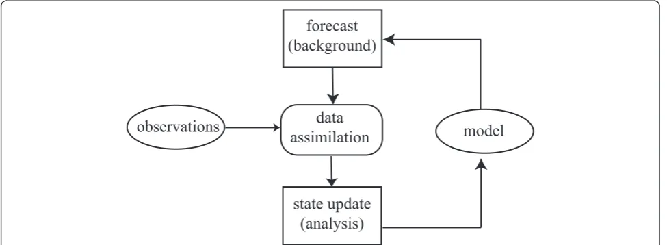
Our approach is derived from one used in numerical weather prediction, illustrated schematically in Figure 1. One begins with a model-generated forecast, often called the background. The chaotic evolution of the weather assures that uncertainties in atmospheric initial conditions grow rapidly with time. To make useful pre-dictions, the background must be updated frequently (typically every 6 hours for global models) with noisy (and sometimes sparse) measurements. The data assimi-lation procedure updates the background in light of the new observations to produce ananalysis, which, under suitable assumptions, is the maximum likelihood esti-mate of the model state vector. The model is restarted from the analysis to produce a new background forecast, usually for 6 hours hence in the case of a global weather model. Data assimilation and model forecasts can be combined intoobserving system simulation experiments to quantify the effect of changes in observation accuracy, type, location, and frequency on the accuracy of numeri-cal forecasts. Section 2.3.3 outlines one state-of-the-art procedure for performing the state update in complex spatiotemporal models.
Two significant difficulties must be addressed in the context of GBM. First, many details of the growth of glioblastoma tumor cells are poorly understood, in con-trast to the motions of the atmosphere, for which there are well-established physical models. GBM tumors com-prise malignant cells with heterogeneous genetic abnormalities and altered metabolism, cysts, cell debris, and vasculature. The patterns by which glioblastomas invade the brain depend on individual growth character-istics and the cytoarchitecture of the surrounding brain tissue.
The second problem concerns the interpretation of magnetic resonance (MR) imaging studies. Magnetic resonance imaging, typically performed at intervals of
several weeks to months, is the principal means by which the growth and spread of GBM are assessed. Patients are injected with a contrast agent to enhance the visibility of the disruption of the blood-brain barrier. Figure 2 shows a typical MR scan of a patient with a newly diagnosed GBM. The enhancing region (of high-est overall intensity) corresponds to the signal from a contrast agent in a dense area of tumor blood vessels. Because these vessels are unusually permeable, the sig-nal probably also reflects contrast agent that has leaked into the surrounding brain tissue. GBM tumors are characterized by profuse abnormal vasculature that is associated with masses of malignant cells, so areas of greatest enhancement are associated with regions of high GBM cell density. Surrounding the central enhan-cing region is an area ofedema (swelling) that also may show some contrast enhancement due to tumoral influ-ences on the surrounding brain tissue, which includes abnormal and permeable tumor vasculature and inva-sion of tumor cells into normal brain tissue [1].
The quantitative relationship between image pixel intensity and tumor cell density is a topic of current investigation. Magnetic resonance images may be manu-ally“segmented”to identify and select those portions of the image that correspond to the actual tumor, edema, etc. Individual variations in brain anatomy, tumor com-position, and tumor mass effect also lead to variability in their interpretation, even among expert assessors. Furthermore, variations in contrast uptake, MR signal, and other aspects of image generation may arise from exam to exam. Thus, some ambiguities may occur when mapping a given set of magnetic resonance images to the brain atlas associated with the dynamical model. The interpretation of MR images may be further com-plicated by treatment: radiation necrosis, for example, may appear similar to new tumor growth [2].
model
observations
data
assimilation
forecast
(background)
state update
(analysis)
The goal of this paper is to establish that, under rea-sonable assumptions, good quantitative predictions of GBM growth and spread are possible, as well as esti-mates of their uncertainty. The discussion is organized as follows. Section 2.1 provides background on GBM tumors and selected mathematical models thereof. Sec-tion 2.2 describes the raSec-tionale for ensemble forecast methods. Section 2.3.3 outlines a modern data assimila-tion algorithm called the Local Ensemble Transform Kalman filter. Section 3 describes the results of its appli-cation in some observing system simulation experi-ments, using magnetic resonance images for estimates of the tumor population density with two different mod-els of the growth dynamics, to establish proof of princi-ple of their utility for potential clinical application.
2 Methods
2.1 Two mathematical models of glioblastoma
Glioblastoma multiforme (GBM) is the most common malignant brain tumor. Despite treatment, patient survi-val is less than 15 months, on average, from initial diag-nosis [3]. GBM tumors are aggressive, largely resistant to chemotherapy and radiotherapy [4], and can quickly invade large and sensitive regions of the brain, making complete surgical resection of the tumor impossible and post-surgical recurrence inevitable [5]. Because little progress has been made against GBM, its biology remains the subject of intense study.
The simulations in this paper involve two mathemati-cal models that attempt to capture the gross dynamics of GBM growth and expansion. Eikenberry et al. [6] suggested a model of four stochastic differential equa-tions whose principal dynamics are the diffusive spread and logistic growth of a proliferating and a migrating set of tumor cells. Swanson and co-workers [7,8] considered simpler models of a uniform tumor cell population. In both cases, the models are simulated on a realistic (but static) brain geometry in which the diffusion rates differ between white and gray matter regions.
In the simplest view, the growth of GBM cells is assumed to be exponential, and their spread is governed by Fick’s Law, which leads to a model of the form [7]
∂g
∂t =∇ ·
D(x)∇g+αg. (1)
The diffusion rate of GBM cells is faster in white mat-ter than in gray matmat-ter; often Dis piecewise constant. The diffusion coefficients, as well as the growth ratea, may be approximated from in vitrostudies, sequential MR studies of individual patients, or the Einstein-Stokes relation [7].
Equation 1 predicts that the tumor cell density can become unbounded. A potentially more realistic model is Gompertzian or logistic growth to some local carrying capacityTmax; in the latter case, the model becomes [9]
∂g
∂t =∇ ·
D(x)∇g+αg
1− g
Tmax
. (2)
Typical values for the parameters in Eq. (2), which we will call the logistic Swanson model, are reported in Table 1. Another model, by Eikenberry et al. [6], divides the cancer cell population into proliferating and migrat-ing classes and also attempts to capture the degradation of the extracellular matrix by the invading tumor. In this paper, we consider a simplified version of the Eikenberry model, which assumes that there is a net transition of cells from the proliferating to the migrating phenotype along the tumor front, gradually degrading the extracellular matrix (ECM).
The net growth of the proliferating cells is logistic (this term also incorporates the net transition from the migrating to the proliferating phenotype as well as cell death due to crowding). The dependent variables are
g(x, t) = proliferating cell density m(x,t) = migrating cell density
w(x, t) = extracellular matrix (ECM) density
and the two-phenotype model is expressed as a coupled set of three partial differential equations, as fol-lows.
∂g
∂t = ∇ · (DG(x)∇g)
diffusion
+αg
1− g+m Tmax
logistic growth − ∇ ·(χ(x)g∇w)
directed migration into ECM
(3)
∂m
∂t = ∇ · (DM(x)∇m)
diffusion
+ ∇ ·(χ(x)g∇w)
directed migration into ECM
(4) Figure 2A representative magnetic resonance image of a GBM
∂w
∂t = −ρw
g+m
θW+g+m
degradation
+αWw(1−w)
repair
(5)
Table 2 displays the nominal parameter values for the two-phenotype model, Eqs. (3)-(5). The values used here differ slightly from those in [6] and were chosen so that the total tumor cell populations from both the logistic Swanson model, Eq. (2), and the two-phenotype model grow at approximately the same rate.
Both sets of equations are integrated using a brain geometry from the BrainWeb database, developed by the McConnell Brain Imaging Center of the Montreal Neurological Institute at McGill University [10]. We use the discrete anatomical model of a normal brain gener-ated for McGill’s MR simulator, which consists of a 181 × 217 × 181 isotropic grid of 1 mm3 voxels in Talairach space [11]. Each voxel is classified as background, cere-bro-spinal fluid (CSF), gray or white matter, fat, muscle/ skin, skin, skull, or glial matter. To reduce the computa-tional expense, the equations are integrated over a representative coronal slice at the center of the 3-dimensional domain, from which voxels representing the skull and other non-brain tissue have been removed. The resulting 2-dimensional domain is a fixed 145 × 143 grid (the mass effect is not modeled). For simulation purposes, glial matter is treated as white matter, and the diffusion coefficients (DG andDM, as appropriate) are piecewise constant.
The spatial derivatives are approximated by finite dif-ferences, and the resulting set of ordinary differential equations is integrated over the 2-dimensional coronal domain using the second-order (in time) Heun’s method
with a fixed time step (0.1 day-1). Given the discrete nat-ure of the brain geometry, location-dependent para-meters (such as the diffusion constants) are taken to be piecewise constant.
[Although a forward integration method for finite dif-ference schemes can be unstable, the authors believe that Heun’s method provides a reasonable compromise between numerical stability and simplicity of implemen-tation for testing the state estimation procedure described here. The robustness of the integration scheme has been tested by halving, doubling, and quad-rupling the nominal domain resolution. In all cases, the 90-day tumor population, integrated from a fixed initial cell distribution, varied by less than 10 percent for suita-bly small time steps (typically 0.05-0.5 day), which was judged satisfactory for our purposes here. Implicit sol-vers require significant effort to implement because the brain geometry induces complicated no-flux boundary conditions; nevertheless, implicit solvers may be required for choices of model parameters that make the equations stiff.]
Figure 3 shows the evolution of a typical GBM tumor under the two-phenotype model, Eqs. (3)-(5), for the nominal parameter values given in Table 2. The initial condition is prepared by integrating a population of 100 growing and 10 migrating cells in a single 1 mm2voxel for 365 days, which under these parameters yields a starting population of approximately 105 cells covering about 150 mm2. The equations are integrated over the indicated 2-dimensional coronal slice for an additional 360 days; snapshots of the tumor cell density at 60-day intervals are plotted in Figure 3. (The axes show the spatial extent of the domain in millimeters.)
Table 1 Representative parameters for the logistic Swanson model, Eq.(2), in two dimensions.
Location-independent parameters Meaning value
a maximum glioma growth rate 0.2 day-1
Tmax glioma carrying capacity 10 000 cells mm-2
Location-dependent parameters Meaning White Matter Gray Matter CSF
D(x) diffusion rate (mm2day-1) 0.0065 0.0013 0.001
Table 2 Nominal values of the parameters for the two-phenotype model, Eqs.(3)-(5), in two dimensions.
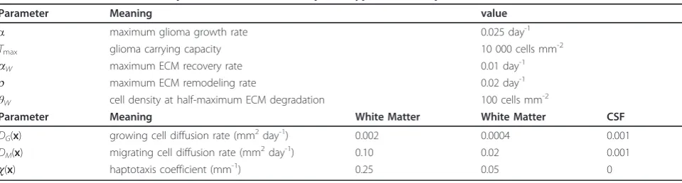
Parameter Meaning value
a maximum glioma growth rate 0.025 day-1
Tmax glioma carrying capacity 10 000 cells mm-2
aW maximum ECM recovery rate 0.01 day-1
r maximum ECM remodeling rate 0.02 day-1
θW cell density at half-maximum ECM degradation 100 cells mm-2
Parameter Meaning White Matter White Matter CSF
DG(x) growing cell diffusion rate (mm2day-1) 0.002 0.0004 0.001 DM(x) migrating cell diffusion rate (mm2day-1) 0.10 0.02 0.001
The bar on the right shows the color coding of cell density: dark blue (lowest density) to dark red (highest density). More precisely, the cell population density is mapped to one of 128“bins,”each of which corresponds to a given color. The darkest blue color corresponds to voxels in which the tumor cell density is between
3
128Tmax and 4
128Tmax, and so on to the darkest red color
where the cell density approaches Tmax. The brain
domain is shown wherever the tumor cell density falls below 1283 Tmax; this color coding is dark gray for gray
matter, white for white matter, and light gray for CSF. We presume that the warmer colors correspond approximately to the enhancing region in an MR scan and cooler colors to a portion of the visible edema; tumor cells are present at a nontrivial density (up to1283 Tmax)in a region extending 2-4 mm beyond
the periphery of the blue-shaded area.
We have chosen the logistic Swanson and two-pheno-type models because they are adequate to establish the potential feasibility of a data assimilation (state estima-tion) scheme in the face of significant errors in model parameters and data acquisition. One must integrate several dozen different initial conditions and parameters in parallel, which can be done in a reasonable period on a multicore laptop computer for these particular models. Both models give plausible simulations of the natural history of a GBM tumor from initiation to diagnosis,
but the omission of mass effect is a limitation, and we do not wish to suggest that one provides a better math-ematical representation of GBM biology than the other. Interested readers may consult [12] for a survey of mathematical models of glioma.
2.2 Ensemble forecasting
In a classic 1963 paper [13], Edward Lorenz showed that a simple model of fluid flow, consisting of three coupled ordinary differential equations, exhibits what is now called chaotic behavior. Such a system is sensitive to small changes in initial conditions: simulations started from states that initially are close together quickly diverge. Although trajectories from typical initial condi-tions (i.e., those that are not fixed points or unstable periodic orbits) appear to approach the same limit set, they become uncorrelated after awhile even when the initial conditions are close together. The implications for weather forecasting are clear: the atmosphere cannot be sampled everywhere, all observations are noisy, and no forecast model is perfect. These factors, with the chaotic dynamics, imply that there is a finite time hori-zon past which weather forecasts are no more accurate than climatological averages.
Even on time scales of a few days or less, uncertainties in the initial state of the atmosphere may lead to sub-stantial forecast errors. In a 1965 paper [14], Lorenz suggested that, instead of running one forecast from a
20 40 60 80 100 120 140
t = 60 days t = 120 days t = 180 days
20 40 60 80 100 120 140
20 40 60 80 100 120 140
t = 240 days
20 40 60 80 100 120 140
t = 300 days
20 40 60 80 100 120 140
mm mm
mm mm
mm
t = 360 days
0.1563 0.3125 0.4688 0.6250 0.7813 0.9375
× Tmax
0.1563 0.3125 0.4688 0.6250 0.7813 0.9375
× Tmax
best guess of the initial state, one should run an ensem-bleof many forecasts, each from a statistically equivalent estimate of the initial state, to give a Monte Carlo esti-mate of the forecast uncertainty for a given weather model. Under appropriate assumptions, the ensemble mean becomes an empirical maximum-likelihood fore-cast. By 1992, supercomputers had become sufficiently powerful to make ensemble forecasting a practical part of the daily operations at the U.S. and European weather centers [15].
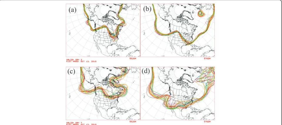
Figure 4 shows representative ensemble forecasts of geopotential height contours at 500 hPa (about half of the mean surface pressure). Each curve shows the result, from one initial condition on Oct. 12, 2010, of a forecast obtained by running the weather model for 3 days (top panels) and 7 days (bottom panels). Roughly speaking, the maps show the predicted locations where half the atmosphere’s mass is below 5520 m (left panels) and 5760 m (right panels). (The geopotential, F(z), is the work needed to raise a unit mass a vertical distance z from mean sea level and accounts for the variation of the earth’s gravitational field with latitude and elevation. The geopotential height isF(z)/g0, whereg0 = 9.80665
m s-2is the global average of gravitational acceleration at mean sea level. For more details, see Chapter 1 of [16].) Of greatest interest here is the forecast uncer-tainty, which varies considerably in space as well as in time. Because of the chaotic dynamics, the forecast uncertainty generally is larger at 7 days than at 3 days. The 5760-m contours (right panels) show considerable
spread over the North Atlantic Ocean at 7 days, corre-sponding to especially large uncertainties in the forecast of the 500-hPa geopotential height.
Unless the initial conditions are updated sufficiently often, numerical weather models produce forecasts that are only as accurate as an almanac’s. Modern opera-tional meteorology relies on state estimation procedures that are based on the Kalman filter, described in Section 2.3.1. The Kalman filter in turn relies on an accurate characterization of the forecast uncertainty, i.e., the cov-ariance matrix associated with the model state vector. Depending on the resolution, a contemporary weather model may have on the order of 106 to 1010 compo-nents in its state vector. The associated covariance matrix is far too large to be stored on a supercomputer, even if one were able to estimate all the elements. Methods to reduce the dimensionality of the estimation problem therefore are essential. A forecast ensemble can provide an empirical, low-rank approximation of the forecast covariance matrix, and spatial localization restricts the scope of the analysis to regions where the forecast dynamics are most highly correlated. (For example, during the 6-hour interval over which weather models are updated, atmospheric conditions over New York and San Francisco are effectively independent.)
The ensemble approach can be adapted to the cancer models, Eq. (2) and Eqs. (3)-(5). Although the logistic terms do not foster chaotic dynamics, the forecast uncertainty increases with time due to errors in the initial tumor population and in the model parameters.
(a)
(b)
(c)
(d)
In addition, the dimensionality problem remains: at 1 mm resolution, the spatial domain for the human brain contains more than 1 million grid points.
The results presented in Sec. 3 are obtained from an ensemble of 50 model realizations of an underlying
“true” tumor, i.e., a tumor whose dynamics are given exactly by Eqs. (3)-(5) with the parameter values in Table 2. For each realization, the growth rateaand car-rying capacityTmax are chosen from uniform
distribu-tions centered about the nominal values in Tables 1 and 2. (Once fixed, they remain constant for the duration of the simulation; Table 3 shows the range of each distri-bution.) In addition, each realization uses a different estimate of the initial tumor density within each grid box (see Sec. 3). The tumor model is integrated to pro-duce a 60-day forecast of the state of the tumor. At that time, we imagine that a new MR image becomes avail-able that provides a noisy observation of the tumor cell population. The Local Ensemble Transform Kalman Fil-ter, described next, updates the forecast ensemble using the MR data. The updated ensemble is used to create a subsequent 60-day forecast, and so on. The process stops if it diverges or if the tumor grows so large as to be fatal.
2.3 Data assimilation
In this section, we briefly describe the rationale and algorithmic implementation of the Local Ensemble Transform Kalman Filter (LETKF) for data assimilation. (See Hunt et al. [17] and Ott et al. [18] for a detailed mathematical justification.) The basic problem may be stated informally as follows: Given a forecast model con-sisting of a coupled system of ordinary differential equa-tions, u˙=F(u, t), find the trajectory u(t) that best fits the observations. In the case of meteorology, the dyna-mical system Fis deterministic, but there is uncertainty in the initial condition,u(t0). (More generally, one can
regard F as having a stochastic component.) Suppose that, fori= 1, 2, . . . ,n- 1, we have a vector of obser-vationsyithat is related to the system state byyi=Hi(u (ti)) + εi, where εi is a Gaussian random variable with mean0and covariance matrix Ri. In the scenario envi-sioned here, theobservation operatorHi(u(ti)) is the MR image that, given a perfect model F in the absence of noise, would result from a tumor whose density in each
grid box isu(ti) = ui. Data assimilation is an application of weighted least squares, as we now describe.
2.3.1 The Kalman filter
We motivate our approach by first considering the case of a linear model,ui=Miui-1, whose observations are a
linear combination of the system state: yi =Hiui +εi. (We follow the development in [17] here.) A maximum-likelihood approach suggests that the “most likely” tra-jectory {ui} is one that minimizes the quadratic cost function
n−1
i=1
(yi−Hiui)TRi−1(yi−Hiui). (6)
The Kalman filter provides an iterative method to compute the minimizer. Suppose that, at timetn-1, we
have a minimizer u¯an−1 =u¯a(tn−1)with an associated
covariance matrixPan−1, that is,
n−1
i=1
(yi−Hiui)TR−i1(yi−Hiui) = (u− ¯uan−1) TP−1
an−1(u− ¯uan−1). (7) One can regardu¯an−1andPan−1as the mean and
covar-iance, respectively, of a Gaussian probability distribution that represents the relative likelihood of the possible sys-tem states given the observations att1, . . . ,tn-1.
Absent further information, the most likely estimate of the system state attnis the model forecast,
ubn=Mnuan−1. (8)
Its associated covariance matrix is
Pbn =MnPan−1M
T
n+Cn. (9)
Under a linear model, a Gaussian distribution of states at timetn-1propagates to a Gaussian distribution at tn.
Model errors increase the uncertainty, which can be approximated by takingCnas a symmetric positive defi-nite matrix.
If a new observation vectorynbecomes available attn, then it can be shown [17] that the relation (7) is satis-fied if the updated state estimateu¯anminimizes
J(u) = (u− ¯ubn)
TP−1
bn(u− ¯ubn) + (yn−Hnu)TR−n1(yn−Hnu). (10)
Equation (11) weights the forecast and the observa-tions. roughly speaking, the minimizer is closer to the
Table 3 Parameter intervals for the forecast model, Eq.(2), used to integrate the ensemble solutions in the observing system simulation experiments.
Experiment 1 Experiment 2 Experiment 3
0.01767≤a≤0.035347 0.0153≤a≤0.0612 0.0153≤a≤0.10
(260 to 520 days) (150 to 600 days) (90 to 600 days)
8000≤Tmax≤12000 8000≤Tmax≤12000 8000≤Tmax≤12000
2.0 × 10⁻³≤Dw≤2.0 × 10
-2
2.0 × 10⁻⁴≤Dw≤2.0 × 10
-2
2.0 × 10⁻⁴≤Dw≤2.0 × 10
quantity with the smaller covariance. The minimizer is
¯
uan=u¯bn+PanH
T
nR−n1(yn−Hnu¯bn) (11)
where
Pan = (I+PbnH
T
nR−n1Hn)−1Pbn. (12)
The matrixPanH
T
nR−n1, often called theKalman gain
matrix, describes how to apportion the discrepancies between the actual and predicted observations to yield the increment between the forecast ("background”) state,
¯
ubn, and its update ("analysis”),u¯an.
Equation (11) shows that it is possible to compute updated maximum-likelihood estimates ofall compo-nents of the model state vector, even if they cannot all be measured, provided that the observations are reason-ably correlated with the model state. For example, sup-pose a Kalman filter is applied to the two-phenotype model, Eqs. (3)-(5), where the state vector u contains components (g, m, w), corresponding to the growing and migrating cell densities, plus the relative density of the ECM, at each point of the domain. Also suppose that it is possible to make noisy measurements only of the total GBM cell density at each grid point. The observation operator, H(u), would then be the predicted value,g+m, of the total GBM cell density at each grid point. Equation (11) shows how to ascribe the difference between the predicted and observed values of total cell density toeach component, (g, m, w), in the update of the grid point in question (and Eq. (12) estimates their covariance), even though the densities of the growing and migrating cells cannot be measured separately. 2.3.2 Variations on the Kalman filter
As mentioned in Section 2.2, one difficulty with a naive application of the Kalman filter is that the covariance matrices of the background and analysis states,Pbnand
Panrespectively, are very large. In addition, the models that we are considering are nonlinear, which implies that the background (forecast) covariance matrix Pbn cannot be computed as a simple matrix product.
There are three overall approaches to the latter pro-blem. One is theextendedKalman filter, which attempts to estimatePbnthrough a suitable integration of a linear-ized model (i.e., the associated variational equations) [19]. The principal difficulty with this approach is that it is highly dependent on the model equations. It is diffi-cult to linearize a large model, and if the model equa-tions change, then so does their linearization. Data assimilation systems based on this approach are tightly coupled to the forecast model.
A second approach is the unscentedKalman filter, in which so-called “sigma points” are chosen about the ensemble mean and integrated with the model to esti-mate the forecast covariance matrix [20]. The unscented
Kalman filter relies on adequate sampling of the error probability distribution, which becomes impractical once the dimension of the model state space is sufficiently large.
The third approach is an application of the Monte Carlo method: run an ensemble of forecasts, as described in Sec. 2.2, to find a low-rank approximation of the forecast covariance matrixPbn. If one can find
sui-table sets of initial conditions from which to integrate the model, then the corresponding forecasts can be used to parametrize (at least approximately) the distribution of the forecast error [19]. The ensemble approach is model independentinsofar as it does not rely explicitly on the model equations; rather,Pbnis estimated empiri-cally from the forecast state vectors.
The ensemble must be large enough to provide an adequate sample of the space of forecast uncertainties. With sufficient sampling, the unscented and ensemble filters should yield the same results as the extended fil-ter. However, the model linearization may be difficult to program, and the integration of the variational equations is computationally expensive. The Local Ensemble Transform Kalman Filter, described next, is an ensemble method. Although it is not a fundamentally new approach to state estimation, extensive tests with com-plex atmospheric models have shown that it is computa-tionally efficient, easily parallelizable, and highly accurate [21,22].
2.3.3 The Local Ensemble Transform Kalman Filter
When the model (or observation operator) is nonlinear, Eqs. (10)-(12) must be modified. The background (fore-cast) covariance matrixPbnis no longer a simple matrix product and must be approximated by other means, as described in Sec. 2.3.2. In addition, the (suitably modi-fied) cost functionJmay have no unique minimizer, and even if one exists, there is no guarantee of optimality, in the sense of being an unbiased estimator with minimum variance. Nevertheless, schemes that seek to minimize cost functions similar to Eq. (10) have proven useful in operational meteorology (see [15] and references therein for an extensive bibliography).
The objective of an ensemble scheme is to choose a set of analysis vectors whose spread aboutu¯anprovides a suitable approximation of the state uncertainty Pbn.
Computational limitations generally restrict the number of ensemble members,k, to be less than a few hundred– much less than the number of state variables in most cases. Nevertheless, if the background ensemble suitably approximatesPbn, then it is possible to generate an
spanned by the ensemble. If the underlying dynamical process has more thankpositive Lyapunov exponents, then an analysis of the form (11) cannot correct forecast errors outside the span of the ensemble subspace.
The LETKF, therefore, is applicable to models that exhibit local low dimensionality–that is, models whose local dynamics over short time intervals can be regarded as relatively low dimensional but driven by the dynamics of neighboring regions [23]. Experience suggests that many geophysical models exhibit this property. The logistic growth term in the GBM models considered here also leads to local low dimensionality: once an initial population of cells invades a given volume of the brain, it grows to an asymptotic value. The region of greatest uncertainty in any GBM forecast is the location of the tumor“front,”as the rate at which GBM cells dif-fuse into healthy tissue may vary significantly with time and location [24].
The idea behind the LETKF is to perform a local ana-lysis that requires the ensemble to capture the forecast uncertainty in only a portion of the state space. Each local analysis involves a separate linear combination of the ensemble solutions over a given local region. In this way, the dimensionality of the global analysis is much larger thank. Extensive investigations have shown that the LETKF is an accurate and computationally efficient data assimilation system for complex geophysical mod-els, including the Global Forecast System, which is the U. S. Weather Service’s operational model [22]; a coastal estuarine model of New York Harbor [25]; and a dyna-mical model of the Martian atmosphere [26], among others.
We briefly outline the implementation of the LETKF used to obtain the results in Sec. 3. The overall objective is to use the observations contained within a suitable local region to update the state estimate of the grid point in the center. In other words, the LETKF finds the minimizer of Eq. (10) one grid point at a time within the subspace spanned by the ensemble solutions. (The
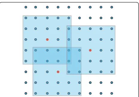
“cookbook” below provides a step-by-step outline.) Fig-ure 5 illustrates the idea schematically for local regions consisting of 5 × 5 grid boxes. In each case, the grid point in the center of the local region (marked in red) is updated using observations located anywhere under the pale blue cover. Because the local regions belonging to adjacent grid points overlap considerably, the set of observations used to update the grid points tends to vary relatively slowly as a function of location, assuming that the observations are sufficiently dense. This prop-erty helps to assure the continuity of the analysis, as explained below. Although the mathematics does not require that the local regions be squares or circles, or even that they be centered exactly on the grid points, it is convenient to define them as such in actual
implementations, except possibly near the boundaries of the model domain. For simplicity of exposition, we refer to the“center”as the grid point being updated by obser-vations in the local region. Each grid point is updated independently, so the computations may be performed in parallel; in this way, the LETKF may be implemented efficiently on modern computers.
The following discussion summarizes the considera-tions and computational procedure that attend to each local region. The global analysis is computed grid point by grid point, using suitable local regions around each. The size of the local regions may be fixed (as in the results reported here) or may vary by location.
Spatial localization As noted above, the dynamics in a
of the region with highest contrast on the MR scan (cf. Figure 2). In the situation described here, the local region size should be comparable to the spatial correla-tion length of the tumor dynamics; since the tumor
“front”is of greatest interest, local regions from 5 mm × 5 mm to 11 mm × 11 mm should suffice. We have used ensemble sizes of 25 and 50 in our simulations with roughly comparable results. Larger ensembles tend to provide better parametrizations of the distribution of forecast uncertainties; the results described in Sec. 3 have been computed with 50-member ensembles.
Ensemble We assume that, at time tn, a set of
back-ground ensemble forecasts,ui
bn, i= 1, 2, . . . ,kis avail-able. Each uibn is a vector containing the full set of model variables over the entire domain. We denote by
xibthe components ofui
bnassociated with the model grid point at the center of the local region. (In Sec. 2.1, we used x to denote a given spatial location within the domain of the PDE models. Here xi
bdenotes the model
state at a particular location. In the case of the two-phe-notype model, Eqs. (3)-(5), xibis the 3-vector (g, m, w) giving the density of proliferating and migrating cells and the extracellular matrix at the grid point in question.)
Suppose that the solution vector at each model grid point containsmcomponents (e.g.,m= 3 in the case of the two-phenotype model) and that there areℓ observa-tions in the local region. Compute the mean,x¯b, of the
ensemble state componentsxi
b,i = 1, 2, . . . ,k, and the
m×kensemble perturbation matrixXbwhoseith col-umn isxi
b− ¯xb.
The LETKF seeks to minimize an objective function ffo the form (10) within the subspace spanned by the forecast ensemble. In other words, rather than finding an estimate of the entire state vector x, we seek a linear combination of the ensemble forecasts that minimizes Eq. (10) for the components of x that correspond to a given local region within the physical grid of the model and that lie in the ensemble subspace. As a conse-quence, the minimizer has the form x=x¯b+Xbw, and
the“cookbook”below shows how to calculatew. One important consideration is that the columns of Xb, by construction, sum to 0 and therefore do not form a basis for the subspace spanned by the ensemble solutions. In particular, the k-vector whose components are 1 belongs to the null space ofXb, so the rank of the k×kensemble covariance matrixPb= (k−1)−1XbXTb is
at mostk- 1. However,Xbis one-to-one on its column space S, so we regard Xb as a linear transformation from an abstractk-dimensional spaceS˜toS and mini-mize J on S, relative to which Pb has a well defined
inverse. It can be shown that if w∈ ˜Sis Gaussian with
mean 0 and covariance matrix (k - 1)-1I, then
x=x¯b+Xbw is Gaussian with mean x¯band covariance
matrixPb[17].
Observations and data selection The observation
operator Hneed not be linear. Only the components within the local region are selected for the analysis. Let
hibdenote theℓvector of the components of the
obser-vation operatorH(uibn)within the local region. Let ynbe the (global) vector of observations. As withH, only the components of the observation vectorynthat belong to the local region (Figure 5) are used; denote them byyo. As with the model state vectors, we let y¯bbe the mean of the vectors hib, i = 1, 2, . . . , kand define theℓ ×k matrixYbwhose ith column ishib− ¯yb. In what follows, we also assume that the observation error covariance matrixRhas been truncated to the observations within the local region.
We assume that H, if it is nonlinear, can be approxi-mated asH(x¯b+Xbw)≈ ¯yb+Ybw. The goal is to find a
linear combination, w, of the ensemble solutions to minimize the cost function
J∗(w) = (k−1)wTw+ [y
o− ¯yb−Ybw]TR−1[yo− ¯yb−Ybw], (13)
which is the analogue of Eq. (10) in the subspace spanned by the spatially localized ensemble solutions [17]. The first term, (k- 1)wTw, represents the forecast uncertainty and has a particularly simple form by virtue of the representation of the ensemble subspace in terms of the perturbation vectors that formXb.
The remaining steps are a“cookbook” recipe for com-putingwand the local analysis ensemble.
1. Compute the k × ℓ matrix C=YT
bR−1. (If the
observations are not independent andRis not diag-onal, it is computationally more efficient to solve the systemRCT=Ybinstead of invertingR.)
2. Compute the k × k symmetric matrix
˜
Pa= [(k−1)I/ρ+ CYb]−1. (See below for more
dis-cussion ofr.)
3. Compute thek×kmatrixW˜a= [(k−1)P˜a]1/2, by
which we mean the symmetric square root. This choice ensures thatW˜adepends continuously on the
elements ofP˜a. (Otherwise, small changes inP˜aat
neighboring grid points can lead to very different analysis ensembles [17,27].)
4. Compute thek-vectorw¯a=P¯aC(y0− ¯yb)and add
it to each column ofW˜ato form the k×kanalysis
weight matrixWa.
6. The analysis ensemble, xi
a, is formed by addingx¯b
to the ith column ofXa,i= 1, 2, . . . ,k.
Global analysis ensembleThe global analysis ensemble,
ui
an, consists of the collection of local analysis ensembles,
xia, at the center of each local region.
Covariance inflation In principle, the only free
para-meters in the LETKF scheme are the ensemble size, k, and the size of each local region. In practice, however, the model is not a perfect representation of the underly-ing dynamics. As a result, ensemble methods tend to underestimate the actual background uncertainty, which causes them to underweight the observations in the ana-lysis scheme. In severe cases, the filter can diverge. One ad hoc remedy is to“inflate” the background ensemble covariance by a tunable parameter. The procedure described above has the effect of multiplying the back-ground ensemble perturbations by√ρ.
2.4 Observing system simulation experiments
In meteorology, tests of proposed data assimilation sys-tems are calledobserving system simulation experiments. Because the weather is a complex multiscale process, one hopes to separate the effects of observation density, location, and error from model error. In aperfect model simulation, one creates a“truth run”from a fixed initial condition with the same model that is used to make the ensemble forecasts. At intervals, synthetic noisy observa-tions are generated from the “truth.” The goal of the simulation experiment is to determine how well a fore-cast ensemble tracks the truth when the synthetic obser-vations are assimilated using a forecast model that is identical to the model used for the truth run [21]. Such experiments can quantify the effect of noise and obser-vation density and frequency on the accuracy of the analyses, since there is no model error. (The assimilation of actual atmospheric observations, of course, provides a test of the data assimilation system in the presence of model error. Since the truth is not known, the analysis quality is assessed using a surrogate, such as the root-mean-square difference between a 48-hour forecast started from the ensemble mean and the corresponding observations.)
In contrast to the usual situation in meteorology, where most of the governing equations of the atmo-sphere are well established, the forecast models consid-ered here are relatively crude approximations of the underlying dynamics. GBM tumors comprise a heteroge-neous population of cells, and, although the tumor as a whole may grow and spread at rates that are reasonably well described by the nominal parameter values, muta-tions among the genetically unstable population may
cause the growth and migration rates to change unpre-dictably from their nominal values.
Furthermore, in a clinical setting, every patient receives treatment (usually some combination of sur-gery, radiation, and chemotherapy), whose effects have not been well characterized in the mathematical models described here. For these reasons, we use different mod-els to generate the observations and the forecasts in the results described below.
2.4.1 Forecast model and ensemble generation
Given the current state of knowledge, errors in any con-temporary forecast model for GBM are likely to be sig-nificant, and we wish to establish the efficacy of the data assimilation scheme under such circumstances. For the observing system experiments described here, we take as the “truth” a tumor whose growth dynamics are sup-posed to be governed exactly by the two-phenotype model, Eqs. (3)-(5), with the parameter values given in Table 2. Synthetic observations of the true tumor con-sist of noisy MR images whose overall intensity is assumed to vary linearly with cell density. They are assimilated at regularly spaced intervals to update an ensemble of initial conditions for which the forecast model is Eq. (2), the logistic Swanson model. A similar model has been used to assess the survival times in indi-vidual GBM patients following surgical resection [9], and it can be integrated readily for many different sets of initial conditions on a laptop computer. (We could just as well have used the logistic Swanson model for the“truth” tumor and the two-phenotype model as the forecast model. Qualitatively similar results would obtain, but the computational expense would be consid-erably greater.)
The filtering scheme described in Sec. 2.3.3 is applied to a 50-member forecast ensemble once every 60 days, and the simulation is continued for 360 days to assess its accuracy and stability. This process is necessarily lim-ited in duration, because the tumor eventually grows to a size that causes fatal complications. No attempt has been made to assess the effect of treatment, which is a subject for future investigation.
Our principal focus is the effect of model and observa-tion uncertainties on the effectiveness of our data
assim-ilation approach. To attempt to capture the
heterogeneity of GBM tumors, we consider an ensemble of models: each ensemble solution is integrated using Eq. (2) with a unique set of parameter values as well as initial conditions. In the results described here, we choose random values within certain intervals of the logistic growth rate a, carrying capacity Tmax, and the
Alternatively, one might allow the parameters to vary with time, possibly according to a random process with drift, but this simple setup suffices to demonstrate the viability of the overall approach.
2.4.2 Generation of synthetic observations
The operator H(x) gives the quantity that would be observed if the tumor state vector were x. As discussed in the introduction, many details of the relationship between tumor cell density and contrast enhancement are not well characterized, and there is intrinsic variabil-ity in contrast agent uptake and other aspects of MR image generation. Hence we assume thatHhas a ran-dom component. For our purposes here,H(x) represents the contrast enhancement (above a baseline level) due to the presence of tumor cells and that the enhancement varies linearly with the tumor cell density at each point of the domain, plus a random value.
The value of His computed pointwise as follows. Let uk(x, t) be the tumor cell density for thekth ensemble member at locationx at timet. Let
hk(x) = max
0, min
1,uk(x,t) Tk
max
+η(x)
, (14)
whereh(x) is a uniformly distributed random value in [-0.1, 0.1] andTk
max is the carrying capacity for thekth
ensemble solution. The value ofhk, which is clamped to the unit interval, is the component ofHcorresponding
to location x in the brain domain. (The h’s are
independent.)
Equation (14) represents an idealized situation, because it ignores the mass effect of the tumor and assumes that there is a one-to-one mapping between pixels in the generated observation and grid points in the model domain. A mathematical characterization of contrast enhancement in individual clinical cases, as well as the registration errors in the mapping between the model domain and MR image, are subjects of ongoing investigation.
2.4.3 Data assimilation and analysis procedure
Each observing system simulation experiment proceeds as follows. Steps 1 and 2 constitute the initialization phase.
1. The “truth tumor” is integrated according to the two-phenotype model, Eqs. (3)-(5), with the para-meter values given in Table 2, to produce the sequence of states shown in Figure 3, which are then used to generate all the observations as described above.
2. An initial ensemble of 50 solutions of the logistic Swanson model, Eq. (2), is prepared by choosing an initial cell density randomly and uniformly from the interval [50,150] in a single voxel within 3 mm of
that used to start the truth tumor. Each ensemble solution has a unique set of model parameters that are chosen randomly and uniformly from the inter-vals given in Table 3; they remain constant for the duration of the simulation. Each single-voxel“seed” is integrated for 365 days and produces an initial tumor of about 105 to 106 cells. Three sets of obser-ving system simulation experiments are performed, using parameters chosen from the intervals listed in the respective columns of Table 3.
3. After the truth and ensemble solutions are pre-pared as described in Steps 1 and 2, the reanalysis phase begins. We assimilate a synthetic MR image that has been generated from the truth tumor according to Eq. (14) and the Local Ensemble Trans-form Kalman Filter is applied as described in Sec. 2.3.3 using a 7 mm × 7 mm local region and a mod-est covariance inflation factor (r= 0.1). The updated ("analyzed”) ensemble solutions are integrated for 60 days to produce a new background forecast.
4. Step 3 is repeated att = 60, 120, 180, 240, 300, and 360 days, for a total of seven assimilation steps and six forecast cycles.
Three such experiments are conducted with forecast model parameters chosen randomly and uniformly from the intervals in Table 3 for the logistic Swanson model, Eq. (2). In the case of purely logistic growth,g’=ag(1 -g/Tmax), one can solve explicitly to find the value of a
for which the time needed forgto increase from 1 per-cent to 99 perper-cent ofTmaxequals a specified value. The
first two lines of Table 3 report those values; for exam-ple, in Experiment 1, the smallera yields an interval of approximately 520 days for the tumor cell density to increase from 0.01Tmaxto 0.99Tmaxand the larger value,
about 260 days. The quantity Dw refers to the value of the diffusion coefficient D(x) in white matter. We take D(x) to be piecewise constant, and its value in gray mat-ter is fixed at the nominal value in Table 1. (GBM cells tend to migrate along white matter tracts [28-30] and the two-dimensional domain chosen for these simula-tions contains considerably more white matter than gray matter.)
Both mathematical models considered in this paper predict that the cell density at every point in the core of a GBM tumor eventually reaches the same constant value, Tmax. Such a situation is biologically suspect (as
leads to the eventual divergence of the filter. In the simulations here, we let Tmax be a random parameter
that is fixed for each ensemble solution. Alternatively, one can let Tmax vary randomly in space. Both choices
prevent the background covariance matrix from becom-ing too ill-conditioned.
3 Results
The goal of the observing system simulation experi-ments here is to shadow the“true”tumor, shown in Fig-ure 3, using synthetic observations and a forecast ensemble as described in Sec. 2.4. Figure 6 shows the results of three assimilation experiments following the final assimilation step att= 360 days. The first, second, and third rows correspond, respectively, to Experiments 1, 2, and 3 in Table 3. The left column, labeled“analysis mean,”shows the ensemble mean after the final analysis step, 360 days after initialization; it is the pointwise average of the fraction of the carrying capacity over all the ensemble members. (The color coding is the same as in Figure 3.) The right column, labeled “free run,” shows the corresponding ensemble means after 360 days when no data assimilation is performed. The middle col-umn shows the pointwise absolute difference between the total cell population in the analysis mean and in the true tumor. At most points, the numerical value of this pointwise difference is generally a few percent ofTmax,
so it is colored dark to light blue.
Figure 6 shows that the performance of the data assimilation system degrades gracefully as the extent of parameter misspecification increases. Even in the worst case (Experiment 3), where the white-matter diffusion rate varies by three orders of magnitude and the logistic growth rate by more than a factor of six in the forecast model, the final analysis provides a reasonably good approximation of the core of the“true” tumor (shown at the bottom right of Figure 3). Although the accuracy of the forecasts in Experiment 3 is considerably poorer than in Experiments 1 and 2, the analysis is reasonably good, but it demonstrates considerable uncertainty regarding the spatial extent of the lowest-density cell distribution.
Figure 7 shows the background forecasts during the last three cycles of Experiment 2 and their correspond-ing analyses att= 240, 300, and 360 days, respectively. The left column shows the mean of the forecast ensem-ble, which is a 60-day prediction started from the pre-vious analysis ensemble. (The color coding, which is as in Figure 3, shows the pointwise mean of the tumor cell density at each point, averaged over the 50 ensembles.) The middle column shows the analysis mean, i.e., the corrected background forecast ensemble after the syn-thetic data are assimilated at the indicated time. The
third column is a “spaghetti plot” showing, for each ensemble solution, a contour plot of where the tumor cell density is one-half the carrying capacity, i.e., 12Tmax.
These contours span a 5-6 mm margin, which gives an indication of the uncertainty in the boundary of the highest cell density. The forecast extent of lowest cell density has a greater span, because we have assumed that the noise in our synthetic MR scans, generated according to Eq. (14), is larger on a proportional basis in low-density regions. This assumption reflects our belief that the boundaries of edematous regions are harder to resolve than those of the tumor core.
Comparable results, not shown here, are obtained when the two-phenotype model, Eqs. (3)-(5), is used as the ensemble forecast model. In this situation, other key parameters, such as the haptotaxis coefficient c(x) and the migrating cell diffusion coefficientDM(x), are chosen from intervals of varying width. The results are also relatively insensitive to the size of the ensemble (for example, an ensemble of size 25 works almost as well) and to the size of the local region (e.g., 5 mm × 5 mm to 11 mm × 11 mm local regions yield approximately similar results).
4 Discussion
This preliminary study demonstrates the potential feasi-bility of ensemble forecasting and data assimilation methods for short-term prediction of the growth and spread of malignant brain tumors. Our principal focus is on the efficacy of a Kalman-type filter for estimating initial conditions from noisy imaging data. Although the immediate application is to glioblastoma, the design and implementation of the Local Ensemble Transform Kal-man Filter (Sec. 2.3.3) do not depend on the particular equations of a given mathematical model. Hence, this forecasting and state update approach may prove useful in other biomathematical investigations.
warrants careful consideration in future efforts to synthesize mathematical models and clinical data for predictive purposes in individual patient cases.
Nevertheless, considerable work remains before our approach can be seriously considered in clinical settings. Many challenges are common to all mathematical simu-lations of cancer [31] and to glioma in particular [32,33]. We outline a few of them here.
The mathematical models
The preliminary investigation here makes no attempt to account for the effects of treatment. The parametriza-tion of any mathematical model of treatment must account for many variables, including the timing and dosage of radiation [12,34], chemotherapy [35], systemic steroids [36], and mass effect [37-39]. Model error. Mathematical forecast models of glioblastoma (and
other cancers) are likely to suffer significant errors, which are treated only crudely in the simulations described here. Improved mathematical characteriza-tions of forecast model error, including model para-meter calibration and more accurate quantification of uncertainties in the state estimate and its covariance in the presence of systematic errors, is a topic of ongoing research [40-42].
Magnetic resonance imaging
The correspondence (if any) between tumor cell density and contrast enhancement in MR images needs to be established. One must assess the variability in opera-tional settings for a clinical scan (including but not lim-ited to magnet strength, pulse sequencing, and the dosage of contrast agent) and the variability among patients (for example, the rate of uptake and metabolism
20 40 60 80 100 120 140
analysis mean free run
mm
mm mm mm
mm
20 40 60 80 100 120 140
20 40 60 80 100 120 140
20 40 60 80 100 120 140
mm
20 40 60 80 100 120 140
analysis mean −truth
20 40 60 80 100 120 140
of contrast agent). Although a statistical predictor of glioma grading based on MR imaging has been pro-posed [43], the authors are unaware of any studies that attempt to relate cell density to contrast enhancement in MR images.
Image registration
Besides the problem of determining the initial density of tumor cells, one needs a geometrical atlas for the model. This can be done using a standard set of such atlases, such as the BrainWeb database [10], or one can attempt to construct an atlas from each individual patient. There is considerable variability even between the brains of healthy people. For example, the brains of men and women differ, on average, in gross total volume and in the distribution of gray and white matter [44]. The mass effect of GBM tumors adds to the diffi-culty. The registration error must be accounted for in
the observation covariance matrices used in the data assimilation procedure.
Non-Gaussianity of data
Finally, to simplify the mathematics, ensemble Kalman filtering schemes assume that the errors in the data and the model are gaussian (or can be adequately approxi-mated by gaussian distributions). The previous consid-erations may result in error statistics that deviate significantly from gaussianity. Future work should char-acterize the error statistics in clinical cases and adapt the minimization strategies in the LETKF accordingly.
5 Conclusions
The Local Ensemble Transform Kalman Filter provides an accurate and computationally efficient way to update the state vector (initial condition) of a complex spatio-temporal model with new quantiative measurements. Its
20 40 60 80 100 120 140
background mean analysis mean
20 40 60 80 100 120 140
20 40 60 80 100 120 140
20 40 60 80 100 120 140
20 40 60 80 100 120 140 20 40 60 80 100 120 140
mm
mm mm
mm mm mm
analysis uncertainty
t = 240 days
t = 300 days
t = 360 days
efficacy relies only on the local low dimensionality of the underlying model dynamics, not on the equations themselves, and so provides a flexible state update scheme even as the models themselves are improved. An accurate forecast system for glioblastoma may prove useful in clinical settings for treatment planning and patient counseling. The model independence of the LETKF provides a flexible framework for other mathe-matical modeling efforts in biology and oncology.
Reviewers’comments
The authors sincerely thank the reviewers for their care-ful reading of the manuscript and their suggestions for improvement. In the reports reproduced below, we have replaced references to page numbers in the review manuscript with section numbers and have omitted comments about typographical errors, all of which we have corrected.
Reviewer’s report 1
Tomas Radivoyevitch, Case Western Reserve University, USA.
This paper is important because the approach pre-sented is generally applicable, and because the notion that states can be observed (i.e. estimated/inferred) even if they cannot be directly measured, needs to receive more attention in biology. This is a very well written paper.
Major compulsory revisions:
One thing the paper could use is a little more clarifi-cation [in Sec. 2.3] regarding how the LETKF is model independent. Specifically, is it that the Kalman gain in Eq. (10) has been replaced by a tuned asymptotic obser-ver matrix that is now merely tuned for algorithm con-vergence kinetics and thus independent of the model? Or, in the simple case of a linear model, is it that the background stateubis somehow no longer Mubn−1i.e.,
somehow now independent of M? It needs to be made clear whether “model independence” means everything is 100% data driven, or whether it means that all possi-ble underlying nonlinear models are reduced to linear models, so it matters not matter what the true underly-ing nonlinear model is (in which case one might argue that the method depends on the linear model that it is reduced to, and thus is not model independent). In the paragraph just before Sec. 2.3, regarding uniform distri-butions centered about nominal values in Tables 1 and 2, please state the range (lower and upper limits) of the uniform distribution used. This should also be done just before Sec. 2.4.2.
Authors’ response: We have attempted to clarify this point by adding a new subsection (Sec. 2.3.2 in this ver-sion of the paper), which motivates the various approaches to Kalman filtering for nonlinear models.
The LETKF, like all ensemble approaches, does not rely on a statically tuned model covariance matrix. Instead, the background covariance matrix, Pbn, is estimated
empirically from the forecast ensemble. Equally impor-tantly, the LETKF also estimates the covariance of the updated state vector in light of the new observations at each step. The variational equations of the model are not needed, and in this respect, the LETKF is a model-independent approach. Our methodology requires that the background and analysis perturbations provide a reasonable local linearization of the dynamical model and observation operator, as described in the discussion in Sec. 2.3.3 leading to Eq. (13). We have added refer-ences to Table 3, which provides the range of parameter values used in the simulations, at the appropriate points in Sec. 2.2 and Sec. 2.4.1.
Reviewer’s report 2
Kristin Swanson, University of Washington, USA (nomi-nated by Georg Luebeck, Fred Hutchinson Cancer Research Center, USA).
This paper illustrates how one might use an estab-lished method of data assimilation, the Local Ensemble Transform Kalman Filter, to update the state vector of a system given new data when modeling glioblastomas. This is done by presenting two different models for glio-blastoma, using one to generate a “truth”with which to update the predictions of the other. Since synthetic data is used, this is clearly a proof of concept and there are many pitfalls this method may incur when attempting to apply this technique clinically. The authors do mention at least some of these. In the field of glioblastoma mod-eling this is certainly a new technique and worth consid-ering. Though, its power would be increased if combined with a technique for patient specific model calibration as well. In general, the paper is well written and presented. There are just a few comments and con-cerns we have that should be addressed.
Comments:
1. While it is not the goal of the paper to assess assumptions of the models used, it should be noted that there is actually a neglible amount of extracellu-lar matrix in the brain.
assumption about a particular physical or chemical form of the brain ECM, which is still in the early stages of characterization. The model simply assumes that there is a generalized barrier that is degraded near the tumor front and promotes inva-sion of tumor cells. We do not assert that the two-phenotype model is a “better” model of GBM than the one-phenotype model; it is used merely as a proxy for a “true” tumor whose internal dynamics are more complex than those represented in a fore-cast model.
Concerns:
1. Section 2.1: In the vast majority of the work done by Swansonet al., the value ofDin the CSF is taken to be 0. Admittedly, this is not mentioned in the 2003 paper or in the 2008 paper, but neither is the value of 0.001 listed. It is not physical for the tumor to grow relative to which PB has a well defined inverse. doubtfully change the proof of concept pre-sented, it should be remarked upon and kept in mind for future use.
Authors’response: We appreciate this clarification. Although tumor cells do not proliferate in the CSF, it seems probable that they diffuse into the CSF at a nonzero rate, hence, a small value for D(x) seemed more plausible to us than a no-flux condition. We agree that the precise value of D(x) within the CSF, as long as it is small, is not likely to significantly affect the dynamics of either model considered here. 2. According to Table 2 and Table 3, the values of Dg, Dm, and Din the CSF regions are all the same value. Thus, the comment in the paragraph introdu-cing the two-phenotype model regarding their rela-tive values seems incorrect.
Authors’response:As mentioned above, we chose small values of these coefficients to reflect a nonzero rate of diffusion into the CSF. The rates are identical for both cell phenotypes because, for the moment, we have no reason to believe that they should be significantly dif-ferent. In both models, the cell diffusion rates are taken to be greater in white matter than in gray matter. 3. In the last paragraph of Sec. 2.3.1 it is said that it is shown in Sec. 3 that “it is possible to estimate the densities of both the growing and migrating cell populations. . .” However, in Sec. 3 it is only men-tioned that it can be done, but never shown. This should either be added as an additional full example or the comment should be modified.
Authors’ response: We have added a paragraph of
explanation regarding this point at the end of Sec. 2.3.1.
4. Figure 5 would better illustrate the method of localization if a third box were added with the center grid point within one of the other regions. That is, it would better illustrate how every grid point is asso-ciated with its own local region if it was illustrated that the“primary”point can be within another local region.
Authors’ response: We thank Dr. Swanson for this
suggestion for improvement, which has been incor-porated into Figure 5 (and its caption).
5. In the Spatial Localization paragraph of Sec. 2.3.2 [now Sec. 2.3.3], it is mentioned LETKF is relatively insensitive to ensemble and local region size vided they are within a reasonable range. Please pro-vide the approximate ranges you tested to give more intuition as to just how insensitive they are.
Authors’response:We have included more details on this point in the discussion in Sec. 2.3.3, which replaces Sec. 2.3.2 in the original manuscript. 6. In the Ensemble paragraph of Sec. 2.3.2 [now Sec. 2.3.3], an example is given for xib as a 4 vector including the a variable for chemorepellent. Such a variable was never introduced in Eqs. (3)-(5). Also, this is inconsistent with the next sentence saying, e. g.,m= 3. It seems the variablecshould be removed. Authors’response:We have made this correction. 7. In the observation and data paragraph of Section 2.3.2 more intuition should be given to the first term of the objective function. It is likely a regulari-zation, but an explicit description should be pro-vided. Also, more intuition for what the“cookbook” is doing would be good. It seems like it should be finding a zero of the derivative of the objective func-tion, but the steps do not give an immediate feel for that.
Authors’ response: We thank Dr. Swanson for this
helpful suggestion and have added a few paragraphs of explanation about this matter in Sec. 2.3.3. 8. Regarding the comments in the final paragraph before the results section aboutTmax. The situation
that the cell density is uniform within the core of the tumor is indeed biologically suspect. But taking Tmaxas spatially variable or as a random parameter
does not seem to be the best way to combat this. In fact, those solutions also seem biologically suspect since it indicates the maximum cells that can occupy a region. A better solution would be to include cell death in the model and allow for a necrotic core (what is actually seen in Figure 2).
Authors’response:GBM tumors are a heterogeneous