N ew D ev elo p m en ts In P rofilo m etric
M easu rem en t
and T estin g o f L arge-O p tic s
A Thesis Submitted for the Degree
of
Doctor of Philosophy of the University of London
by
Lee Hubbard
Optical Science Laboratory
Department of Physics and Astronomy
University College
ProQuest Number: 10106500
All rights reserved
INFORMATION TO ALL USERS
The quality of this reproduction is dependent upon the quality of the copy submitted.
In the unlikely event that the author did not send a complete manuscript and there are missing pages, these will be noted. Also, if material had to be removed,
a note will indicate the deletion.
uest.
ProQuest 10106500
Published by ProQuest LLC(2016). Copyright of the Dissertation is held by the Author.
All rights reserved.
This work is protected against unauthorized copying under Title 17, United States Code. Microform Edition © ProQuest LLC.
ProQuest LLC
789 East Eisenhower Parkway P.O. Box 1346
N e w D ev elo p m en ts In P rofilom etric
M easu rem en t
and T estin g o f Large O p tics
A b stra ct
This thesis is mainly concerned with the development of a profile measuring instru
m ent, to work in the 1 m eter plus diameter area of large optical production, with a
resolution in the tens of nanometers region. Development of such an instrum ent also
addresses an im portant area of optical testing which is concerned with the testing
of complex and difficult optical surfaces, which cannot be tested with traditional
optical test methods.
The thesis starts with a historical review of profile measuring instrum entation,and
continues to discuss the optical production and test facilities available at the Optical
Science Laboratory, (OSL) . A study of the optical specifications of 8 m eter class
telescope secondary mirrors has used to develop a specification of resolution and
dynamic range leading to development of the instrum entation.
The main part of the thesis discusses the development of a number of different
instrum ent components. The three m ajor components are discussed in this the
sis. A new type of laser reference system, which uses a laser beam in free air, in
combination with a custom designed actuator flexure and software control system,
defines an absolute reference plane for measurement. A new type of interferometric
measurement system, is used as a surface height measurement, as well as an axis
position measurement system, to define measurement coordinates. The last area of
instrum ent development, adressed by the thesis is the development of a low contact
force surface probe system, based on a torsion wire.
The thesis concludes with a series of system testing culminating in a test on a toroidal
surface, which is classically difficult to test. The performance of the system is then
reviewed against the specifications initially determined earlier in the thesis. In
conclusion this thesis provides some ideas for future development and improvement
C o n ten ts
1 In tro d u ctio n 17
1.0.1 The Schmaltz R eco rd er... 18
1.0.2 The Contorograph ...18
1.0.3 The Tomlinson Surface Recorder ... 19
1.0.4 The A bbott P ro h lo m eter... 20
1.0.5 The Talysurf ... 20
1.0.6 Limitations of Early Contact P r o h lo m e tr y ... 22
1.1 Optical Production at O S L ... 24
1.2 Optical Testing At OSL ... 26
1.3 Defining A New I n s t r u m e n t ... 33
1.4 An Outline of the Prohlometer P r o j e c t ...37
1.4.1 Interferometric Measurement S y s t e m ... 38
1.4.2 A Contact Probe S y ste m ...39
1.4.3 A Laser Reference S y s t e m ...40
1.4.4 The Selection Of laser S o u r c e ... 41
1.5 Summary of T h e s i s ... 41
2 Laser S y ste m s for P rohlom etry. 43 2.1 In tro d u c tio n ... 43
2.2.1 Characterisation of Transition P r o c e s s e s ... 45
2.2.2 Spontaneous and Stimulated Emission P r o p e r t i e s ...45
2.2.3 Polarisation C h a r a c te r is tic s ...47
2.2.4 The Einstein Coefficients... 47
2.2.5 Oscillation Conditions Inside Laser S y s t e m s ...48
2.2.6 Conditions For Optical G a i n ...50
2.2.7 Coherence L e n g th ... 51
2.2.8 Standard Model 1, ’’Two Level System” ... 52
2.2.9 Standard Model 2, ” Four Level System” ... 52
2.2.10 Laser Beam G e o m e tr y ...54
2.3 Gas Laser Systems...56
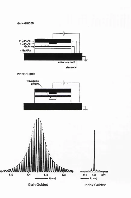
2.4 Semiconductor Laser S y s t e m s ... 59
2.5 Laser E x p e rim e n ta tio n ... 64
2.6 D isc u ssio n ... 68
3 In terferom etric M easu rem en t S y stem s 72 3.1 In tro d u c tio n ...72
3.2 Comparison of Selected Interfero m eters... 73
3.2.1 The Michelson In te rfe ro m e te r...74
3.2.2 Twyman-Green Interferom eter...76
3.2.3 The Jam in I n te rfe ro m e te r... 77
3.2.4 The Mach-Zehnder Interferom eter...79
3.2.5 S u m m a r y ...80
3.3 Optim isation of Interferometer Design ... 81
3.3.1 Selection of m a te ria ls ... 82
3.3.2 Effect of splitting ratio on system p erfo rm an ce...83
3.3.4 The Effects of Optical A lig n m e n t... 92
3.4 Experimental Michelson Interferometers ...92
3.4.1 Michelson Interferometer Prototype 1 ...94
3.4.2 Michelson Interferometer Prototype 2 ...96
3.4.3 The Liquid Reference S u r f a c e ...98
3.5 Multiple O utput Channel Interferom eters...99
3.5.1 Q uadrature O utput Interferometer Prototype 1 ...106
3.5.2 Q uadrature O utput Interferometer Prototype 2 ...107
4 R eferen ce Surface G en eration 116 4.1 In tro d u c tio n ...116
4.2 Concept of a Nulling S y ste m ...117
4.2.1 Effect of Varying Laser Beam P r o f i l e ... 119
4.3 Experim entation W ith Optical F ib e r s ...121
4.3.1 Characterisation of Optical F ib e rs ...122
4.3.2 Experim entation with Fiber Optic C o u p lin g ... 125
4.4 Hardware Based Laser Reference S y s t e m ... 129
4.4.1 System O v e rv ie w ...129
4.4.2 Hardware E lec tro n ics... 131
4.4.3 Flexure Motion S y ste m ... 137
4.4.4 System Performance and T e s t i n g ...139
4.5 Software Based Laser Reference S y ste m ...147
4.5.1 System O v e rv ie w ...150
4.5.2 Actuators For The Compensation Of B a c k la sh ... 151
4.5.3 Actuator Driver E le c tr o n ic s ...157
4.5.4 A ctuator Software C o n tr o l...162
4.5.6 System Testing and P e r fo r m a n c e ... 179
4.6 D iscu ssio n ...182
5 In stru m en t Stru ctu re A nd C on stru ction 185 5.1 In tro d u c tio n ...185
5.2 An Investigation Into Profilometer Support Structures ...186
5.2.1 Round Section Beam And Guide S y s te m ... 186
5.2.2 Double Rail Carriage W a y ... 188
5.2.3 Round and Flat Section Combination Carriage W a y ... 189
5.2.4 Selecting a Carriage W a y ...190
5.3 Support For The Granite Air B e a rin g ...199
5.3.1 Investigation of I-Girder P r o p e r tie s ... 200
5.4 The Effect of Environmental Conditions on Instrum ent Performance . 210 5.4.1 Effect of Temperature Level, Constancy and Uniformity . . . .211
5.4.2 Effect of V i b r a t io n ... 213
5.5 General Instrum ent C o n s tru c tio n ...220
5.5.1 Laser Reference Mounting and Optics A sse m b ly ... 222
5.5.2 Contact Probe S y s t e m ...227
5.5.3 Laser Reference Flexure System and Isolation Electronics . . . 240
5.5.4 Laser Reference End b lo c k ... 242
5.5.5 Interferometer Detection Electronics ... 244
5.5.6 System A sse m b ly ... 245
6 S y ste m T estin g 248 6.1 In tro d u c tio n ...248
6.2 Determ ination of Interferometric Operation... ... 249
6.2.2 Software Based Fringe C o u n t e r ... 253
6.2.3 Summary Of R e s u l t s ... 260
6.3 Determ ination of DSP O p e r a t i o n ... 260
6.3.1 Comparison of DSP System with Heidenhein P r o b e ... 262
6.3.2 Repeatability M e a s u re m e n t... 268
6.4 Optical Profile M easu rem en t... 273
6.4.1 Testing Toroidal Test Plate ... 273
6.4.2 Use Of Test plate In Toroid T e s tin g ...275
6.4.3 Initial Profile M easu rem en ts...279
6.4.4 Higher Density Profile Measurement ... 283
6.4.5 Summary of Results ... 289
6.4.6 Comparison with Instrum ent S p e c ific a tio n ...290
7 C on clu sion s 292 7.1 Summary of Project ... 292
7.2 Instrum ent P e rfo rm a n c e ...293
7.3 Implications and A p p licab ility ...293
L ist o f F igures
1.1 The Schmaltz R ec o rd er... 19
1.2 The Shaw C o n to ro g ra p h ...20
1.3 The Tomlinson Surface Recorder ... 21
1.4 The Abbott P ro filo m eter...21
1.5 Photograph of a Production Model T a l y s u r f ... 22
1.6 Resolutions of Typical Surface Characterisation T echniques... 23
1.7 Installation of the Former Grubb-Parsons Fabrication Equipment . . 25
1.8 Schematic of a Typical Scatterplate Interferom eter... 26
1.9 A Typical Scatterplate Interferogram...28
1.10 OSL Scatterplate Interferometer During Surface Testing ...29
1.11 Contact Profilometer Model 1. [Kim, 4 8 ] ...30
1.12 Contact Profilometer Model 2, [Kim, 4 8 ] ... 32
1.13 Profile of the Gemini Telescope Project Secondary M irro r...34
1.14 Variation in Height Profile for a Tolerance of ± lm m in R ... 35
1.15 Variation in Height Profile for a Tolerance of ±0.0005 in K ... 36
1.16 Variation of Surface Slope for the Gemini Secondary Mirror ...37
2.1 Radiative Recombination P ro c e s s e s ...46
2.2 Spontaneous Emission S p ectru m ... 46
2.3 Idealised Laser C a v i t y ... 49
2.5 Power Verses Pum p R a t e ... 55
2.6 Transverse Laser Oscillation M o d e s ...55
2.7 Propagation of the T E Mqq M o d e ...56
2.8 Simplified Circulatory Laser System Schem atic... 57
2.9 O utput Oscillation m o d e s ...59
2.10 Homo-junction Laser S y ste m ...61
2.11 Cross-Section Through Hetro-junction Laser S y ste m ...61
2.12 Semiconductor laser C h a ra c teristic s...63
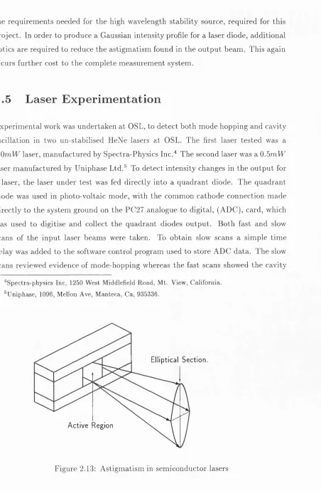
2.13 Astigmatism in semiconductor l a s e r s ... 64
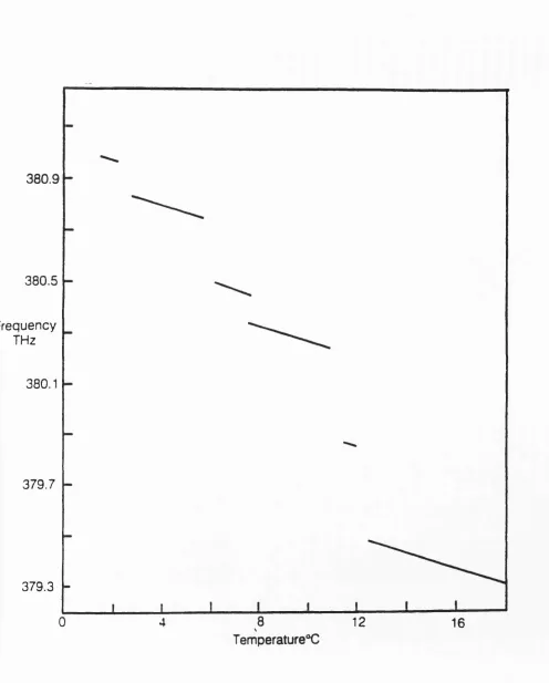
2.14 A typical variation of diode wavelength verses tem perature, [Williams, 8 0 ] ...65
2.15 Effect of Back Reflections on Laser Diode Performance, courtesy of SeaStar Optics I n c ...66
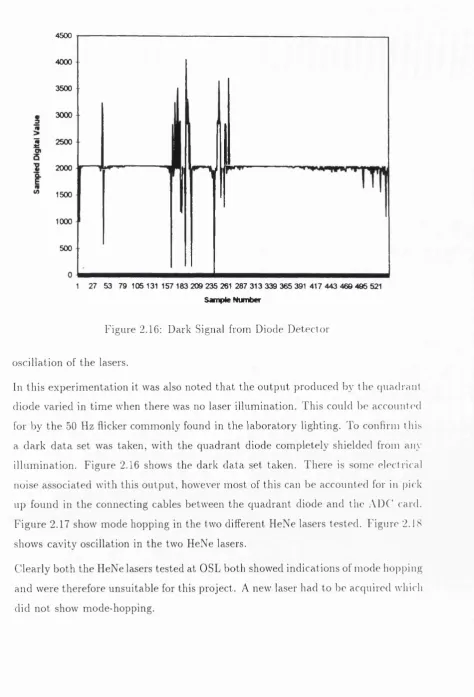
2.16 Dark Signal from Diode D e t e c t o r ...67
2.17 Slow scan showing laser mode h o p p i n g ... 68
2.18 Fast scan showing laser cavity o s c illa tio n ...69
2.19 ML2000 Frequency Drift D a t a ... 71
3.1 Michelson Interferometer S ch em atic...74
3.2 Typical Interference fringes produced from Michelson Interferometer . 75 3.3 Twy man Sz Green in te rf e r o m e te r ...76
3.4 Jam in Interferometer S c h e m a tic ... 78
3.5 Mach-Zehnder Interferometer S c h e m a tic ...79
3.6 Transmission Profile for Crown Glass, Courtesy Spiers Robertson Ltd 83 3.7 Reflectance of an Aluminium Coating, Courtesy Spiers Robertson Ltd 84 3.8 Reflectance of a Protected Aluminium Coating Courtesy Spiers Robert son Ltd ... 85
3.10 Beam Splitter Reflection/Transmission P rofiles...87
3.11 Polarisation Tests on Non-Polarising Beam S p litte rs ... 89
3.12 In p u t/O u tp u t Beam Positions During Retro-Reflector Tests ...90
3.13 Results From Internal Reflection R etro-R eflector...91
3.14 Displacement of O utput Beam vs Angle of Incidence ... 93
3.15 Michelson Interferometer Prototype 1 ... 95
3.16 Schematic of Resultant Fringes ... 96
3.17 Experiment in Interferometer Tilt E r r o r s ...97
3.18 Experimental Floatation S y ste m ... 98
3.19 Experimental Liquid Reference Surface Interferom eter... 100
3.20 Results obtained from Liquid Reference surface Interferometer . . . .101
3.21 Determination of Signal Direction for a Single O utput Channel . . . .1 0 2 3.22 Determination of Signal Direction for Quadrature O u t p u t s ...103
3.23 Determination of Signal Direction for Quadrature O u t p u t s ...104
3.24 Determination of Signal Motion at a Turning P o i n t ...105
3.25 Q uadrature O utput Interferometer Experimental Prototype 1 ... 106
3.26 Results Obtained From Prototype 1 ...108
3.27 Polarising Interferometer Optical L a y o u t ... 109
3.28 Fringes Produced Using Micrometer A d ju stm e n t... I l l 3.29 Interferometer Experimentation B lock...112
3.30 Motor Micrometer driven interferometer s y s t e m ... 113
3.31 Fringe Signals for Different Motor Micrometer S p e e d s ...114
3.32 Calculation Of Signal P h a s e ... 115
3.33 Noise Levels Before and During Fringe M o v e m e n t... 115
4.1 Quadrant Photo-diode Nulling S y s te m s ...118
4.3 Examples of Optical Fiber Construction ... 123
4.4 Four Lowest LP Fiber Oscillation M o d e s ... 124
4.5 Variation of Fiber Attenuation with Input W a v e le n g th ...125
4.6 Comparison of O utput Speckle for Single and Multi-mode Fibers . . . 126
4.7 Experim entation to Couple 50//m Core Optical F ib e rs ... 127
4.8 Point Source Fiber Launch S y s t e m ... 128
4.9 Fiber Optic Beam P ro file...129
4.10 Hardware Based Nulling System O v e rv ie w ...130
4.11 Actuator Power Amplification S ta g e ...131
4.12 Initial Calculation Electronics For Null S ig n als... 132
4.13 Hardware Oscillation Experimental R e su lts...134
4.14 Quadrant Diode Buffer A m plifiers...135
4.15 Monitoring System Interface E le c tr o n ic s ... 136
4.16 Flexure Motion System for Hardware Driven Nulling S y s te m ... 138
4.17 Initial Testing of Hardware Based Control S y s te m ...141
4.18 Measurement of Lower Limit Using a C C D ... 143
4.19 Recorded Error Signal Using The Monitor S o ftw a re ...144
4.20 Relation Between the Error Signal And The Physical E r r o r ...145
4.21 Measurement of Lower Limit Using slip G a u g e s ... 146
4.22 Error signal vs Physical Error, Experiment 1 ...148
4.23 Error signal vs Physical Error, Experiment 2 ...149
4.24 Error signal vs Physical Error, Experiment 3 ...150
4.25 Software Controlled Laser Reference System O verview ... 151
4.26 High Voltage PZT S u p p l y ... 158
4.27 High Voltage Control C irc u it... 160
4.29 DC Motor Micrometer Driver Electronics for Use with a PC24 DAC
C a r d ...162
4.30 Summary of Switching Modes for DC Motor Micrometer Driver Elec tronics ... 163
4.31 LVDT Calibration C u r v e ...166
4.32 PZT Extension for Variable Control v o lta g e s... 167
4.33 Straight Line Fits for Compensation of PZT H y s te re s is ...169
4.34 Motor Micrometer Displacement for Varying Software Loop Cycle Number For The Vertical A x is ... 171
4.35 Motor Micrometer displacement for Varying Software Loop Cycle Number For The Horizontal A x i s ... 172
4.36 Recorded Digital Error Signal for a Square Wave Control Signal . . . 174
4.37 Relation Between Physical Displacement and Recorded Digital Error. 175 4.38 Sequence of Operations for the Main Software Control Program . . . 176
4.39 Software System Test on Vertical Flexure A x is ... 180
4.40 Test Results for the Software Controlled Nulling S y s t e m ...181
4.41 Experimental Software Controlled Nulling System and Associated Measurement Interferometer M o d u l e ... 184
5.1 Support Beam and Carriage System used by [Harrison, 3 9 ] ... 187
5.2 Double Rail Carriage Way S c h e m a tic ... 189
5.3 Round and flat Section Carriage W a y ... 190
5.4 Effect of Roll Motion on the Straightness of Carriage T r a v e l ... 193
5.5 The Effect of Yaw Carriage Motion on Traverse S tra ig h tn e s s ... 194
5.6 The Effect of Pitch Motion On Carriage Position A c c u ra c y ...195
5.7 Effects of Waviness and Roughness on Surface F o r m ...196
5.8 Air Bearing Carriage Way After Assembly at O S L ... 197
5.10 Standard I-Girder Node D is tr ib u tio n ... 201
5.11 An Example ANSYS Model of a Standard I-Girder Under Load . . . 202
5.12 Maximum Deflection for Steel and Aluminium I-G irders...204
5.13 Maximum Girder Deflection Under Applied L o a d ...206
5.14 G ranite/I-G irder Cross-Section Nodal M o d e l... 207
5.15 An Investigation into Reducing Support Structure F l e x u r e ... 209
5.16 Variation of Laboratory Temperature in OSL Optics S h o p ... 212
5.17 Optical Science Laboratory Im Polishing M a c h in e ...214
5.18 Optical Science Laboratory 8 f t Grinding/Polishing M ach in e... 214
5.19 Typical Background Vibration Trace Obtained from Im Machine . . . 215
5.20 P artial Function Fit for Low Order sin(na;) + Bn cos{nx) Terms . . 216
5.21 Fourier Transform of (top) A nsin(nx), (bottom) BnCos{nx) ...218
5.22 Fourier Transform of (top) An sm{nx)-^Bn cos(na:), (bottom ) An sin(æ)”+ Bn cos(a;)” ... 219
5.23 ANSYS4.4A Reduced Harmonic Analysis of Flexure S y s t e m ... 221
5.24 Results of Reduced Harmonic Analysis on Flexure S y s t e m ... 222
5.25 Schematic of Individual Construction Areas ... 223
5.26 Laser Reference Mounting and Carriage Position Optics Assembly . . 224
5.27 Laser Reference System Positional Adjustment M o u n tin g ...225
5.28 Laser Reference Launch System and Carriage Position Interferometer 226 5.29 V-Block Vertical Probe Slideway... 228
5.30 Glazier Bearing Probe Slide w a y ... 230
5.31 Experimental Results Obtained from an Inclined Optical Flat . . . . 232
5.32 Variation of Horizontal Probe Tip P o s itio n ...233
5.33 Low Contact Force Torsion Wire Probe Head ... 234
5.35 Slotted Opto-switch H o u sin g... 237
5.36 Experimental Surface Contact Circuit 1 ...239
5.37 Repeatability of Stopping Position For Circuit 1 ...240
5.38 Experimental Surface Contact Circuit 2 ...241
5.39 Repeatability of Stopping Position for Circuit 2 ...242
5.40 Laser Reference System and Isolation E le c tr o n ic s ... 243
5.41 Laser Reference Flexure and E le c tr o n ic s ... 244
5.42 Interferometer Detection and Signal Adjustment E le c tr o n ic s ...246
5.43 The Prohlometer Measurement Hardware Mounted on the Air Bear ing C a rria g e ... 247
6.1 Schematic Layout of the Hardware Based Fringe C o u n te r ... 251
6.2 Comparison of Heidenhein O utput with Calculated Displacement Deal 253 6.3 Residual of Deal - Heidenhein O utput for Hardware S y s te m ... 254
6.4 Software Driven Fringe Counting Experimental S c h e m a t i c ... 255
6.5 Determination of Counting Level for Software Fringe Counting . . . . 256
6.6 Action of Programmable Software S w itc h ...257
6.7 Comparison of Heidenhein Probe System with Software Driven Fringe C o u n t e r ...259
6.8 Residual of Deal ~ Heidenhein Probe O utput for Software System . . . 259
6.9 Comparison with Heidenhein System for 16th Interpolation Level . . 263
6.10 Residuals for 32 Interpolation L e v e l... 266
6.11 Residuals for 128 Interpolation L e v e l ... 267
6.12 Residuals for 256 Interpolation L e v e l ... 268
6.13 Repeatability for 32 Interpolation L e v el... 270
6.14 Repeatability for 128 Interpolation L e v e l...271
6.16 Optical Test used in Calibrating Test Plate Radius of Curvature . . . 274
6.17 Effect of Manufacturing Error on Test plate P r o f i l e ...276
6.18 Use of Test Plate in Toriod M a n u fa c tu re ... 277
6.19 Effect of Radius of Curvature Tolerance on Toriod Surface Eorm . . . 278
6.20 Side 2 Measurement Set 1 ...281
6.21 Side 2 Measurement Set 2 ...282
6.22 Higher Density Profile Measurement ... 285
6.23 Results of De-trending and Z e r o in g ... 287
6.24 Best Fit Sphere for Profile R e su lts... 287
6.25 Profile Comparison of Measured Profile to Specification Profile . . . . 288
6.26 Residual for Comparison of Best Fit Sphere to Measured Results . . . 289
List O f T ables
1 Comparision Of PZT Manufactures 156
2 LVDT Calibration Results. 165
3 Deflection Of Structural Steel. 203
4 Deflection Of Aluminium. 203
5 Maximum Deflection For Varying I-Grider Dimension. 205
6 ISA Enviromental Guidelines. 210
7 Common Vibration Sources 213
8 Digital Fringe Counter Experimental Results. 252
9 Software Fringe Counter Experimental Results. 258
10 DSP Comparision Results Extending. 263
11 DSP Comparision Results Retracting. 264
12 DSP Repeatibility. 269
13 Standard Deviation Of Repeatibility. 272
14 Initial Toroidal Data, Set 1. 280
15 Initial Toroidal Data, Set 2. 280
C h a p ter 1
In tro d u ctio n
The need to characterise and label items into classes is at the very root of civilisation.
From the earliest times, objects were classified by such variables as weight, size, and
texture. Selecting the correct objects could literally mean the difference between life
and death. W ith the advance and development of civilisations, the characterisation
of m aterials has gradually moved away from such simple properties. The advent
of the industrial age, has seen an acceleration in the need to perform a variety of
classifications and in the importance of these classifications. However, with the need
to classify things comes the problem of how to classify.
Throughout history, there has been an interest in the classification of metals. Ini
tially this was for the purposes of creating weapons, such as swords and knifes.
However, as technology has progressed and manufacturing techniques grown, there
has been an increasing demand to characterise manufactured surfaces.
The effects of scratches and machine marking, specifically on the fatigue strengths of
m etals was being increasingly investigated from 1918 onwards, [Dagnail, 18], chiefly
in connection with the design of aircraft and aero engines. The low weight needed by
these early aircraft meant that propeller shafts and other highly stressed components
m ust have maximum strength, with the minimum of redundant material. Exami
nation of surfaces by microscope and interferometry, although useful, was of rather
lim ited value in this research. W hat was needed was a m ethod of displaying a mag
nified cross-section of a surface. Obtaining cross-sectional information, or profiles,
in this field.
The development of surface profile characterisation instrum entation has continued to
grow since the first instrum ents were constructed. Originally, early instrum entation
was developed upon the idea of recording surface details by direct interface to the
surface under test. This was normally done with a probe or stylus system. Such
measurements could be defined under the prefix of contact measurement, indicating
th at direct contact between the measurement instrum ent and the test surface is made
during a measurement. The first profilometric contact measurement instrum ents
became available in the second half of the 1920’s, [Dagnall, 18], some of which have
been summarised in the following sections.
1 .0 .1
T h e S c h m a ltz R e c o r d e r
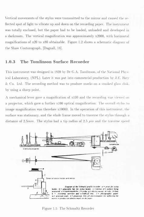
Figure 1.1 shows a schematic diagram of the Schmaltz recorder, [Dagnall, 18]. In
the operation of this instrum ent, a beam of light was reflected from a mirror,c,
connected with the stylus, and focused as a spot onto a roll of photographic paper,
I. The photographic paper was driven past the recording aperture, k, by an electric
motor.
The surface, d, was traversed under a chisel-shaped stylus, / , at around 2m m I sec,
by another motor, g. Vertical movements of the stylus caused the mirror to tilt, with
the result th at the spot of light moved up and down the recording aperture, by this
means a magnification of the irregularity heights of up to x200 could be obtained.
An image of the graticule, m, was also projected on to the photographic paper
and appeared superimposed on the profile trace. The second mirror was deflected
at intervals by the electromagnet, to provide marks on the paper representing a
horizontal scale.
1 .0 .2
T h e C o n to r o g r a p h
Another profile recorder which used an optical lever and photographic recording was
the Shaw Contorograph. The beam carrying the stylus at one end and a mirror at
Vertical movements of the stylus were transm itted to the mirror and caused the r('-
flected spot of light to vibrate up and down on the recording paper. The instrument
was totally enclosed, but the paper had to be loaded, unloaded and developed in
a darkroom. The vertical magnification was approximately x2000, with horizontal
magnifications of x20 to xSO obtainable. Figure 1.2 shows a schematic diagram of
the Shaw Contorograph, [Dagnall, 18].
1 .0 .3
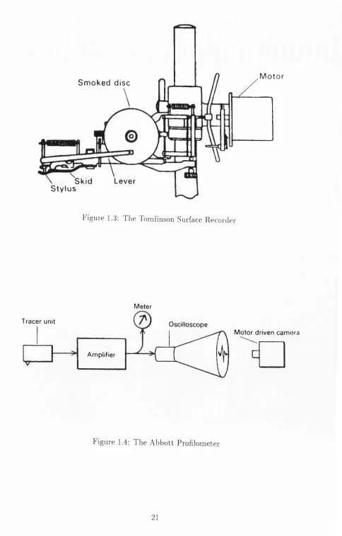
T h e T o m lin so n Surface R e c o rd er
This instrum ent was designed in 1939 by Dr G.A. Tomlinson, of the National Tli\s-
ical Laboratory, (NPL). Later it was put into commercial production by .LIT Maty
& Co. Ltd. The recording method was to produce marks on a smoked glass disk,
lyy using a sharp point.
A mechanical lever gave a magnification of xlOO and the recording was \ iewed on
a j)rojector, which gave a further xlOO optical magnification. The o\erall stylus to
image magnification was therefore xlOOOO. In the operation of this instrum ent, tlie
surface was stationary, and the whole frame moved to traverse the stylus through a
distance of 2.5????n. The stylus had a tip radius of 2.5 ///?? and the traverse speed
••
U r a t i c u l * p r o j t c t O f
D m i a i l o l s l y l u ; h o l d e i « n d m i r r o r
Diofram o f the Stkm ahz profile recorder a = pivot for ttyhts holder, b = adjustable bar for stylus holder r = mirror, d = surface being measured, e * traversing device, f ' ’ stylus, g - electric motor h = slit, i ^ letu - ^ k = recording aperture m d cylindrical lens I = photographic paper. t „ = graticule scale, n = projection lens, p - elrctromagnei for deflecting the
m i r r o r to produce an identttv m a r k on the p a p e r
was 0.01 i m n / s t c . F ig u r e 1.3 shows a. s c h e m a t i c of t hi s i n s t r u m e n t . [Dagnall. 18].
1 .0 .4
T h e A b b o tt P r o filo m e te r
In 1936, the first commercial instrum ent using an electrical transducer ]fickup, called
the Profilometer, came onto the market, [Dagnall, 18].
This instrum ent employed a moving coil pick-up, which traversed across the sur
face by hand. The profile was displayed on the screen on a cathode-ray tube. A
perm anent record could be obtained by simply photographing the cathode-ray tube
screen. Vertical magnifications of up to x50000 were obtainable. An A.C voltm eter
measured the o u tput from the amplifier, and provided a reading of the RMS value of
the profile waveform. Figure 1.4 shows a block diagram of the Abbott Profilometer.
[Dagnall 18].
1 .0 .5
T h e T a ly su rf
R.E. Reason, of Taylor, Taylor and Hobson started a major research project into
th e nature and measurement of surface finish, [Reason, 64, 65]. The result was the
first of a long, still continuing, line of Talysurf instruments.
Dr Reason’s work laid the foundation for standardising surface texture m e a su re m e n t.
b oth nationally and internationally. Talysurfs went into commercial production in
1942. Figure 1.5 shows a photograph of a production Talysurf produced by Rank
M o t o r
S m o k e d disc
Skid Lever St yl us
Figure 1.3: The Tomlinson Surface Recorder
M eter
Tracer unit
Oscilloscope
M o to r driven cam era
A m plifier
Figure 1.4: The A bbott Profilometer
P a r a m e t e r s e l e c t c M a g n i f i c a t i o n s w i t c h T r a v e r s e
! u n i t
D i s p l a y
A m p l i f i e r £t p r o c e s s o r
u t - o ff s e i e ^ t o
R e c o r d e r
Figure 1.5; Photograph of a P roduction Model Talysurf
Taylor Hobson. ^ The hrst of these instrum ents incorporated most of the m ajor
basic features of subsequent versions. A discussion of the use of a Talysurf is given
by [Spragg, 70].
1 .0 .6
L im ita tio n s o f E arly C o n ta c t P r o filo m e tr y
As previously discussed, early contact profilometry was based upon the need to
obtain surface information for aeronautical engineering applications. T he typical
resolutions th a t could be obtained were within engineering tolerances, ranging from
to 5/.W2. At the tim e of the production of this instrum entation, these reso
lutions were acceptable, since components could not be machined to b e tte r than
these tolerances. However with the progression of m anufacturing technology, there
has been a dem and for higher accuracy surface measurements. W ith instrum ents
like the Talysurf range, the measurement resolutions available have been substan
tially refined to the point where sub-micron resolutions are available for engineering
applications.
A nother of the problems associated with early contact profilometry, if com pared
to more recent instrum entation, was the problem of surface damage incurred
dur-^Rank T aylor H obson, N ew star R oad , T h u r m a sto n L ane, L eicester, E n glan d .
ing a surface measurement. The main cause of this damage was the liigh contact
forces present in the measurement instrument. W ith the ability to produce better
quality m anufactured surfaces, the effects of surface contact force has become an
increasing concern, [Wills-Moren and Leadbeater, 81]. This concern has led to the
parallel development of non-contact profilometric technology. A typical example of
non-contact profilometry is the work of [Ophey, 58]. The majority of non-contact
profilometric instrum entation relies on interferometric measurement systems, where
the surface under test forms the moving arm of the interferometer. There is how
ever an inherent problem with non-contact methods th a t use this system. To obtain
an acceptable percentage of light reflected from the measurement surface, the m ea
surem ent surface must firstly be partially reflective. Although, this problem can
be alleviated by using a grazing incidence system. Secondly, the measurement sur
face must possess low surface roughness of typical value less than the illuminating
wavelength, to avoid scattering of the incident interferometer measurement beam,
[Bennett 6]. These problems limit the use of non-contact profilometric instrum ents
to the late stages of surface production.
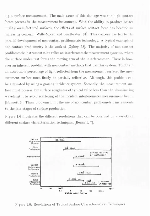
Figure 1.6 illustrates the different resolutions th a t can be obtained i)V a \'ariety of
different surface characterisation techniques, [Bennett, 7].
E lectro n M ic ro s c o p e
(S tereo)
Stylus P ro filo m eter
In te rfe ro m e te r
l 2 0 - 1 5 0 0 X l
kI - 1 0 « m t
( 1 0 - 2 5 0 o X |
D E P E N D S O N T Y P E
O f I N S T R U M E N T
O p tic a l H e te ro d y n e P ro filo m eter
O p tic a l P ro filo m eter
Total I n te g r a te d
S c a tte rin g
(4 -loooXi
l 5 0 o X - 1 0 . m (
IS - 3 5 o X r m i t
H i i o o X - I h e i g h t s
\ I I U N R E S O L V E D
10 100 JOOOX 1 lO m m
0 1 I 1 0 1 0 0 lOOOu m
S P A T I A L W A V E L E N G T H S
Figure 1.6: Resolutions of Typical Surface Characterisation Techniques
1.1
O p tic a l P r o d u c t io n at O SL
The UK has a history of being one of the world leaders in the manufacture of large
optics for astronomical applications. The reputation of UK optical manufactures
has been established over a number of decades, and is typified by such names as
Grubb-Parson & Co. Ltd.
In 1984, Grubb-Parsons & Co. Ltd was closed by its controlling company NET
Parsons Ltd. The production personnel and expertise located at the former Grubb-
Parson fabrication facilities were dispersed after the closure. The former technical
manager of Grubb-Parson, the late Dr D. Brown, relocated to the University of
Durham, taking the m ajority of the former Grubb-Parson test optics. He had been
employed as a consultant of OSL, to document a technical record of large optics
production at Grubb-Parsons. However this relationship was cut short when Dr
Brown died suddenly in 1987. The death of Dr Brown was a great loss for large
optics production nationally in the UK, and indeed world-wide.
It was realised by Dr D.D Walker ^ and Dr R.G Bingham ^ th at it was very im portant
for the UK to retain the expertise in the production of large optics, so th at the
UK could successfully contribute and compete in technical proposals involving the
production of large telescope optics.
In 1987, plans were put forward, by OSL, to carry out work in the field of large
optics production. Contact was made between OSL, and Grubb-Parsons controlling
company, NEI Parsons Ltd, for the purchase of a Im polishing machine and a. S f t
diamond milling and polishing machine, from their previous locations at the former
Grubb-Parsons factory. Extensive work was carried out on both the installation,
m aintenance and upgrading of these machines at OSL, in order th at both machines
could be restored to the working order they were in previous to the closure of Grubb-
Parsons. Extensive modernisation has also been carried out on the 8 f t machine
to develop computer controlled profile generation, [Kim, 48]. Figure 1.7 shows a
photograph of the 8 f t milling/polishing machine during installation at OSL.
Also, with the kind co-operation of the University of Durham, a large selection of
^Dr D .D W alker, Head o f th e O p tical Science Laboratory
Figure 1.7: Installation of the Former Grubb-Parsons Fabrication Equipment
the test optics taken there by the late Dr Brown was procured. This included ma jor
pieces such as a 30 inch diameter flat and sphere, plus 40 inch and 60 inch meniscus
lenses, for testing convex telescope secondaries, and a Grubb-Parsons wavefront
shearing interferometer. The acquisition of these optics, some of which are unique
world-wide, strongly enhanced OSL’s ability to produce large optics.
In 1988, an extensive research programme was initiated in the active production of
large optical surfaces with the aim to, (I) Produce better quality optics for astro
nomical applications, (2) Reduce the production cost in large optic manufacture, (3)
Reduce the strong link between optical manufacturing and the skilled craftsm an, (4)
Produce further developments on the former Grubb-Parsons polishing technology.
Work in these areas was carried out by a number of OSL personnel, and subsequently
M I R R O R
P R O J E C T I O N S C A T T E R - L E N S P L A T E
P I N H O L E D E F O C U S
T I L T
B E A M S P L I T T E R
MA GE L E N S
I M A G E P L A N E
Figure 1.8: Schematic of a Typical Scatterplate Interferometer
1.2
O p tical T esting A t OSL
The large optical production facilities acquired from Grubb-Parsons, and the sub
sequent work carried out by Dr Kim, [Kim, 48], and others, has resulted in OSb
having the ability to produce large optics up to 2.5 m in diameter.
T he production of optical surfaces normally involves an interative process between
polishing and testing. The ability to test an optical surface during production
provides the m anufacturer with information on the evolving surface, which can be
fed back into the next stage of polishing. Often, it is found th a t the testing of an
optical surface is the ultim ate limiting factor on the form and quality of the surface.
At OSL, there are currently two methods of characterising large optics in the pro
duction stages. The first of these methods is by direct optical testing. A typical
exam ple of such a test is the scatter plate interferometer.
The scatterplate interferometer, commonly in use today, was first conceived by .l.M
Burch, [Burch, 10], in 1953. Figure 1.8 shows a typical optical layout for the scat
te rplate interferometer, [Rubin, 68].
The scatterplate is constructed using photographic techniques. Typically, a beam
from an Argon laser, is scattered by a section of ground glass onto an emulsion
be several wavelengths of path difference in height, therefore minimal direct light is
transm itted through the ground glass onto the emulsion. The result of the ground
glass is a speckle pattern. The emulsion is then double exposed with a 180° rotation
between each exposure, for an equal tim e period. The accuracy to which the rota
tion of the emulsion is achieved and the equality of the exposure times determine the
accuracy of symmetry between the two emulsion components of the scatterplate. Er
rors generated in the symmetry of the scatter plate will degrade the resultant fringe
contrast of the scatterplate interferometer, although a tolerance in rotational error of
about SOArcseconds will have negligible effects on the interferometer performance,
[Rubin, 68].
In the operation of the scatterplate interferometer, the theoretical aspects of which
have been explained by [DeWitte, 23] and by [Houston, 41], the incident light source,
in the case of the OSL scatterplate interferometer a HeNe laser source, when en
counters the scatterplate forming two beams, an unscattered beam, and a scattered
beam. From figure 1.8 there is double passage through the scatterplate, resulting in
four difference component beam amplitudes. The four component beams are formed
as follows,
1. (Unscattered-Unscattered, U-U). The incident light is unscattered in both pas
sages through the scatterplate.
2. (Unscattered-Scattered, U-S). The incident light is unscattered in the first
passage, and scattered on the second passage.
3. (Scattered-Unscattered, S-U). The incident light is scattered in the first pas
sage, and unscattered in the second passage.
4. (Scattered-Scattered S-S). The incident light is scattered in both passages
through the scatterplate.
These four component beams combine and form the interferogram in the image
plane. The component beam formed by the U-U component beam forms the satura
tion spot, normally associated with scatterplate interferometry. The S-S component
adds a constant background intensity to the resultant interferogram. The fringe
Figure 1.9: A Typical Scatterplate Interferogram.
S-U beam components. Figure 1.9 shows a typical interferogram ol)tainecl using a
scatterplate interferometer, [Rubin, 68).
T he results from this instrum ent are normally analysed, at OSL, using WYKO
Phase 2 ” fringe analysis s o f t w a r e . A resolution of A/10 is obtainable, however with
suitable modifications to this system, using phase stepping technology, a theoretical
resolution of A/100 is possible. Figure 1.10 shows a photograph of t his instrument
during surface testing at OSL.
C urrently at OSL there is an F ratio, defined by the focal length of the optic divided
by the diam eter, of F3, above which testing by scatterplate interferometry is not
possible. Although optics with a lower F ratio have been tested, [Rubin, 68], there
is a lim itation inherent to the scatterplate system when testing low F /nos, or high
F / nos. For low F / nos, there is a problem of scatter profile, uneven illumination of the
test optic, and non-isoplanatism, causing a fringe contrast reduction. Isoplanatism is
defined as each pair of symmetrical points on the scatterplate producing an ident ical
fringe p a tte rn in the image plane. For large F/nos, a bright hot spot can be generated
which can wash out a significant portion of the fringe pattern, by increasing the
scattering efficiency, this problem can be alleviated.
T h e second m ethod by which production optics, at OSL, can be characterised is
A w KO fringe an aly sis s y s te m s , W Y K O Corp ora tion, 2650 E .Elvir a R oad, T u cson , Arizona.
Test Optic
/ t . :
a e g : T r ' . ' f "
Scatterplate
4
HeNe Source
Figure 1.10: OSL Scatterplate Interferometer During Surface Testing
profilometric testing. It was demonstrated in a very simple form by Dr Kim. [Kim.
•18). th a t profilometric testing could ultimately be useful in the very early si ages
of optical production. However, the resolution th a t can be obtained using profilo
m etric instrum ents can be compared to the resolution obtained from optical tests.
[Church, 16). The size of optics which can be measured using profilometric methods
is dependent upon the nature of the equipment used. Prior to the project discussed
in this thesis, two simple contact profilometers were developed by [Kim, 48). These
instrum ents are summarised below.
1.2.0 . 1 C o n ta c t P ro filo m ete r M odel 1
T he aim of this profilometer was to assess the profile of milled surfaces, generated
using the 8 ft milling machine at OSL. In the construction of this profilometer. a
Im optical flat provides the reference plane for measurements. linear velocity
differential transducer, (LVDT), [Hordeski, 40], provides the probe transducer used
to m easure the height of a surface under test, with respect to the reference plane
provided by the optical flat. Such systems are also discussed by Wills-moren and
Leadbeater, [Wills-Moren and Leadbeater, 81). These height measurem ents are then
Carriage, (Aluminium)
Optical F lat
Optical F lat Support 150mm
1060mm
LVDT Probe
Optic
Side View
205mm
670mm
Optic
m m
/
Machine TableEnd View
Figure 1.11: Contact Profilometer Model 1. [Kim, 48]
T h e repeatability of the LVDT transducer system is about l ^ m , which is within
th e accuracy required for milled surfaces. This is especially true if it is considered
t h a t up to 20^m of glass material can be removed during loose abrasive lapping.
However the LVDT must be calibrated to measure profiles to within an accuracy of
10//m. During profile m easurement, the LVDT has a continuous motion across the
optic surface. Readings from the LVDT are sent via a RS232 serial link to a PC.
To move the LVDT carriage assembly, across th e test surface, the 8 f t m achine’s
quill was used. The quill is fitted with an X position. Moiré Fringe encoder. From
the work carried out by [Kim, 48] a LVDT positional accuracy of 18/^m could be
non-linearity associated with the LVDT. This is especially true if the LVDT is used
over a large range.
1.2.0.2 C ontact P rofilom eter M od el 2
When the surface quality of optical surfaces approaches the standard where polishing
can be started, it is necessary to obtain profile information to a higher resolution. A
second profilometer was developed to obtain higher resolution profiles, which could
also be used as an additional cross check on the profiles taken with the previous
model 1 profilometer, as well as providing information during the early stages of
polishing.
The second profilometer developed at OSL was also of surface contact type. An
Invar rod formed the support frame for a series of ten LVDT probes, positioned
at precisely determined locations along the length of the Invar support rod. Each
LVDT could be pre-set to a height which conforms to the mirror sag, to the order
of I m m . This was done by placing the profilometer on an optical flat, and using
slip gauges under each LVDT to set the height. This m ethod reduces the dynamic
range used for each LVDT to a much smaller value than compared to profilometer
model 1 and therefore reduces the effects of non-linearity by the LVDT. This is the
key advantage to profilometer model 2 over model 1.
This profilometer was designed to stand on the mirror surface using two support
legs at both ends of the Invar rod. The separation of the legs was 830mm. The
LVDTs used in this profilometer had better repeatability and lower therm al effects
th an the LVDT used in profilometer model 1. Typically, the worse case total error,
estim ated to be of the order of ±5//m , [Kim, 48]. Figure 1.12 shows a schematic
diagram of this profilometer.
1.2 .0 .3 L im itation s o f th e E x istin g P rofilom etric S y stem s
The main aim of these profilometers was to provide a feed back mechanism during
the milling process, by providing surface form information. This information could
then be fed back into the milling process, therefore enabling mechanical errors in
Control Electronics
58mm
Side View
865mm
Knife Edge
LVTD Probe
Instrum ent Support Arm
Invar Rod
End View
Figure 1.12: Contact Profilometer Model 2, [Kim, 48]
The two existing profilometers, at OSL, were both capable of producing acceptable
results to feed back into the milling process. However both show limitations in both
accuracy and dynam ic range. Profilometer model 1 has a m axim um range in X-
position of Im . This is the size of the optical flat used as a reference. Also th e X
encoder used to obtain LVDT positional information does not cover the full dynam ic
range of 2.7m, which is the m axim um capacity of the 8 f t machine. Therefore, if a
larger optic has to be produced, a new reference fiat and X encoder m ust be used
to cover the size of these larger mirrors. However, for profilometer model 2, larger
with one of longer dimension.
The dynamic range in the measurement direction, associated with model 1, is tied
to the range of the LVDT transducer. If optics with sags greater than the dynamic
range of the LVDTs are to be figured, then profilometer model 1 cannot be used
without modification. Profilometer model 2 overcomes this problem by allowing
the vertical positions of the LVDTs to be adjusted to conform with the mirror sag,
although both profilometers suffer from non-linearity in the LVDTs.
The contact force between the probe and the optical surface in both model 1 and
model 2 profilometers was of the order of tens of grams. When very smooth surfaces
are to be measured, low contact forces are required to prevent surface damage.
The accuracies obtained from these profilometers was also low. Although, for the
measurement of profiles during the milling and early polishing stages their perfor
mance is adequate. However for fine figuring and surface quality measurements,
these profilometers are incapable of producing the high measurement accuracies re
quired. Therefore, to obtain the higher accuracy profile information, required in
later production stages, a different additional instrum ent must be used.
1.3
D e fin in g A N e w In str u m e n t
The aim of this project is to develop a new profilometric instrum ent to work in
the area of large optical production at OSL. The specifications required for this
new instrum ent are defined by the optics likely to be measured. To quantify these
specifications a study was performed using the dimensions of a specific telescope
optic. The optic used to quantify the specifications for this project was the Gemini,
[Osmer, 59], telescope project secondary mirror. The Gemini telescope project is a
collaboration between 6 countries, to build two 8m telescopes, one based on Mauna
Kea in Hawaii and the other based at Cerro Pachon in Chile. A profile of the
secondary mirror for the Gemini project can be defined by the following expression,
[Augustyn, 3].
O p t i c H e i g h t (m)
-0 . 0 0 5
-0 . 0 1
-0 . 0 1 5
- 0 . 0 2
- 0 . 0 2 5
-0 . 0 3
-0 . 2
D i s t a n c e F r o m C e n t r e (m)
Figure 1.13: Profile of the Gemini Telescope Project Secondary Mirror
W here Z is the profile height, R is the paraxial radius of curvature, K is the conic
constant, and r is the distance from the optical axis. The values for K and R are
as follows, [Anon, 1].
• r = 1.022 m maximum diameter.
• K = -1.6129 ± 0.001
• R = -4193.069mm ± 5mm
The resultant profile for this optic, at ideal values of R or / i , is shown in figure
1.13. From figure 1.13, the specifications in both vertical and horizontal travel can
be defined. The optic has a vertical sag of about 31mm from the centre to the outer
edge. If a profilometer is required to take a height profile across the whole optic, in a
single profile recording, it must have a minimum vertical dynamic range of 31 mm.
Also, to take a complete height profile, the profilometer must also have a horizontal
range of at least 1.0 2 2m
There is a tolerance associated with both the values of R and K and these tolerances
H e i g h t D i f f e r e n c e (m)
- 6 7
6 . 10
— 6
5
4
- 6 3
— 6
2
- 6 1 . 1 0
-0 . 2 0
0 . 4 0 . 2 0 . 4
R a d i u s O f O p t i c (m)
Figure 1.14: Variation in Height Profile for a Tolerance of ±1?7777?. in R
variation in the resultant profile. If a profilometer is to be used to characterise a
surface, then the resolution required by the profilometer must be better than tlie
deviation caused to the profile by variables used to characterise the profile. If the
profilometer resolution is lower than the deviation in surface form, caused 1)y tlie
tolerances in the defining variables, then the profilometer will not be able to correctly
determ ine whether the surface conforms to its specifications. Ideally the profilometer
should have a higher resolution than the surface form variation it is attem pting
to measure. One way of obtaining the required resolution for the measurement
instrum ent is to tighten the tolerances on R and K and then calculate the required
resolution for these new higher tolerances. The new tolerances for R and K were
set to ÜTTim and ±0.005 respectively.
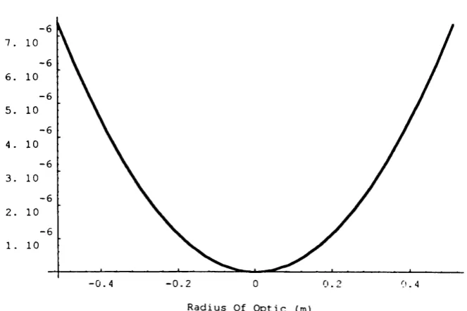
A tolerance of ± lm m in R produces the variation in height profile shown in figure
1.14. The tolerance of ±0.0005 in the value of K produces the variation in height
From figures 1.14 and 1.15, the new tolerance on the values for R and K gives
a sagittal range of ±7.4/zm and ±57nm respectively. Therefore the measurement
accuracy required for the vertical height component is about ±57717??..
The required horizontal measurement accuracy is dependent upon the maximum
slope present in the surface. In the case of the Gemini telescope project secondary
mirror, this is found at the periphery. By differentiating the defining equation for
the mirror surface, the slope of the surface can be found. This is shown in figure
1.16, which indicates a the slope at the periphery is 6.97°.
This gives a required horizontal measurement accuracy of about 47077 7??. For surfaces
of lower slope, the horizontal measurement accuracy can be relaxed substantially.
A summary of the required dynamic ranges and measurement resolutions is shown
below.
• Horizontal dynamic range > 1.022???
V a r i a t i o n O f H e i g h t (m)
10
- 8
D i s t a n c e F r o m C e n t e r (m)
• Vertical dynamic range > 31mm
• Horizontal measurement resolution % 470nm
• Vertical measurement resolution % 57nm
1.4
A n O u tlin e o f th e P r o filo m e te r P r o je c t
The profilometer research project was initiated in 1992 to investigate and construct
a new profilometric instrument to work in the area of large optical production at
OSL. At the time OSL did not have suitable profilometric test instrum entation. The
operation principle for development of a new instrument involved taking a series of
height measurements, with respect to a straight reference plane, at a series of point s,
selected by the user, across a surface, therefore allowing the user to construct a t wo
dimensional profile of the surface under test. The principle of operation for this
S u r f a c e G r a d i e n t
0 . 0 5
-0 . 2
D i s t a n c e F r o m C e n t r e (m
- 0 . 0 5
project differs from surface mapping techniques, as only two dimensional data is to
be taken.
In later development, it is hoped to further develop the operating principle to allow
continuous profile recording of surfaces, to become another option for surface testing.
A num ber of OSL members have been involved in this project since its start, includ
ing the author. A number of different areas of research have been undertaken since
the start of this project, however the project was divided between two main areas of
research. The first area of research was to develop a digital signal processing system,
(DSP), capable of both fringe counting and interpolation, [Mohan, 56]. The second
area of research, was mainly carried out by the author, comprised of research in the
following areas.
• The development of an interferometric system.
• The development of a new type of reference of straightness.
• The design construction and testing of a low contact force surface contact
probe system
The author also carried out extensive work in the area of system construction and
testing of the prototype instrum ent. The following sections discuss the selection of
individual techniques for the research areas the author has undertaken.
1 .4 ,1
I n te r f e r o m e tr ic M e a s u r e m e n t S y s t e m
W hen defining a measurement system it is im portant to understand to what ref
erence the measurement system is calibrated. The overall accuracy of calibration
determines, in-part, the maximum resolution of the measurement system. Any vari
ations in the reference medium during calibration of the measurement system will
be reflected in the overall performance accuracy of the measurement system. For
example, when constructing a Moiré Fringe system, [Guild, 34, 35] and [Chaing, 14],
the accuracy to which the grating lines are ruled sets an upper limit on the reso
lution available to the Moiré Fringe system. Similarly with a LVDT probe system,
calibration of the transducer output to a linear form relies upon the quality of the
One way to reduce errors formed in the calibration of a measurement system is
to design the measurement system about a fundamental invariant, or a pseudo
invariant, th at has a variation far below the desired accuracy of the measurement
system. One such pseudo-invariant is the variation in wavelength of a stabilised
laser system. A measurement system th at could use this principle is interferometry.
A single design for an interferometric system is also capable of operation over the
different dynamic ranges present in this project. If this is compared with a Moiré
Fringe system, a single design could not be used for both dynamic ranges. Another
advantage of an interferometric system is the low, but not negligible, resultant effect
of environmental variations, such as tem perature and humidity. This is of course
assuming th at the correct selection of construction m aterials and component con
figuration is made. W ith other measurement systems this may not be the case. An
example of environmental influence on a measurement system is the performance of
an LVDT transducer under a fluctuating tem perature environment.
Therefore a single interferometer design was developed th at could function over both
the vertical and horizontal dynamic ranges present, and also have minimal variation
in performance due to external environmental influences.
1 .4 .2
A C o n ta c t P r o b e S y s t e m
It was anticipated th at any new profilometric instrum ent would be used in conjunc
tion with the production testing of new optics at OSL. In the production stages, the
surface quality of an optic ranges from a rough milled state, in the initial stages of
figuring, to a finely polished state, in the late stages of production. There are two
m ethods of obtaining information from a surface. Either contact measurement, such
as a LVDT probe, or non-contact measurement, such as a scatterplate interferome
ter. However, in the early stages of optical production it is both extremely difficult
and expensive to test rough ground surfaces using non-contact methods, [Kiichel
and Wiedmann, 49]
Later in the production of an optic, as the surface quality improves, non-contact
surface characterisation does become possible. However, contact measurement is
therefore, depending upon the nature of the contact measurement instrum entation
used, contact measurement can be used throughout the production of an optic.
It was decided th at a contact measurement system should be developed. If a contact
measurement system is to be used to characterise such a surface, it must not cause
damage to the very surface it is attem pting to measure. The contact measurement
system should also be designed in such a way as to facilitate its use on a number
of different optical materials and surface quality conditions. In the later stages of
optical production, as previously stated, the surface quality is very high. At this
stage the surface is very sensitive to defects such as scratches or pits.
One way to reduce the likelihood of surface damage is to design the measurement
probe to have a low contact force. This is the method used in this project to protect
surfaces. A contact probe system was designed to operate on a contact force of <
Im^r, (chapter 5). Positional information, for this probe system, is provided by an
interferometric system, previously designed.
1 .4 .3
A L a ser R e f e r e n c e S y s t e m
Traditionally profilometric instrum entation has relied upon high quality optical fiats
to provide a reference datum for height measurements, [Stedman, 71]. However this
has resulted in large construction costs for this type of instrum entation. It was
recognised th at this is one of the major disadvantages of traditional profilometric
instrum entation.
One of the design aims of this project is to remove the link to high quality reference
flats. To this end, a new laser reference system was developed, (chapter 4). In this
system a laser beam, propagating in free air, is used to define a straight line datum
for subsequent height measurements. A quadrant diode position sensing system,
with associated electronics and software, is used to direct control signals to two
pairs of custom actuators, mounted upon a two axis flexure system. The position
of a height measurement module is controlled by the position of the axis flexure
1 .4 .4
T h e S e le c t io n O f la se r S o u r c e
The design of the profilometric instrum ent for this project makes extensive use of
both interferometric and optical systems. The illuminating source used in conjunc
tion with these systems has a crucial effect on the performance of the instrum ent. In
the case of this project, a laser system has been selected to provide the illuminating
source. However, the interferometric and the optical systems, such as the laser refer
ence system, require slightly different enhanced performances from different aspects
of the lasers performance.
The interferometric systems require high stability in both wavelength and coherence
length, whereas the laser reference system requires a high stability in the pointing
direction and laser oscillation mode. The coherence length required for this project
is about 2m, and is defined by the horizontal dynamic range.
The performance of a laser system is dependent upon many variables, therefore
research was performed into laser technology, culminating in the selection of a laser
source, (chapter 2).
1.5
S u m m a r y o f T h e s is
This thesis presents the work carried out by the author in the design, construc
tion and testing of a new profilometric instrum ent for OSL. Chapter 2 discusses the
im portant variables associated with the operation of lasers, detailing experiments
carried out by the author on the existing laser measurement systems available at
OSL. This chapter ends with the selection of a laser for use in both the interfer
ometric systems and the laser reference system, used in this project. In chapter
3, interferometric systems are discussed. This chapter details experiments carried
out by the author when investigating the available interferometer configurations.
The culmination of this chapter is the construction and testing of a new type of
interferometer. Chapter 4 discusses the construction and testing of two types of
laser reference system, one m ethod based on a purely electronic hardware system,
the other based on a completely software driven system. The results obtained from
instrum ent structure, then details individual construction areas, culminating in a
discussion of the m ajor components for the instrum ent. Chapter 6 presents the
testing of the new instrum ent with respect to its ability to obtain meaningful profile
information. Chapter 7 summarises the implications of the test results discussed in