Spectral Control
A th esis su b m itted for th e degree o f D o cto r o f P h ilosop h y
in E lectron ic and E lectrical E n gineering
March 1997
Sim on Fragiacom o
UCL
ProQuest Number: 10055383
All rights reserved
INFORMATION TO ALL USERS
The quality of this reproduction is dependent upon the quality of the copy submitted.
In the unlikely event that the author did not send a complete manuscript and there are missing pages, these will be noted. Also, if material had to be removed,
a note will indicate the deletion.
uest.
ProQuest 10055383
Published by ProQuest LLC(2016). Copyright of the Dissertation is held by the Author.
All rights reserved.
This work is protected against unauthorized copying under Title 17, United States Code. Microform Edition © ProQuest LLC.
ProQuest LLC
789 East Eisenhower Parkway P.O. Box 1346
This thesis is concerned with channel coding. Channel coding consists of error
control coding and line coding (LC). The basic definitions and concepts of both
error correcting codes (ECCs) and LC are initially examined, followed by the pre sentation of a number of existing coding algorithms. Where appropriate, computer
simulation is used to establish their limitations. Certain new codes are then devised
which offer improved performance.
Finally, following on what is now an established trend, error correcting and line
codes are combined to form error correcting line codes (ECLCs), which may offer superior performance compared to the use of a cascaded scheme.
Specifically, the first chapter contains some basic definitions, the thesis outline
and a summary of the contributions.
Chapter 2 introduces the basic concepts behind error correcting codes and soft decision decoding (SDD) together with a brief description of the well-established Chase algorithms. Their advantages and limitations will be examined and used
generate novel SDD algorithms in chapter 5.
The basic concepts of line coding are introduced in chapter 3. In addition, a
new family of single added bit line codes is also presented. This offers reasonably
good line characteristics with very small compromise to rate.
Chapter 4 is concerned with simulation as a means of evaluating the perfor
mance of coded systems. A conventional simulation technique is initially presented
simulating the very low error rates of modern communication systems, especially
when SDD is used. Two novel simulation acceleration algorithms are therefore
introduced to alleviate this problem. These will only simulate code words th at
affect the residual bit error rate (RBER) and simply calculate the effects of the code words which are correctly decoded. The novel simulator algorithms are used
in subsequent chapters to determine the performance of the proposed new codes.
Chapter 5 introduces the new generalised Chase (GO) algorithms, followed by the adaptive immediate decision (AID) and test pattern elimination (TPE) algo rithms. These can be used to offer near maximum likelihood (ML) performance with minimum increase in complexity.
Chapter 6 is concerned with combined EC and line codes to form ECLCs.
These can offer both tight line coding characteristics and good decoding perfor
mance. Some emphasis is placed on implementation appropriate to very high bit
rate systems.
Finally chapter 7 brings the thesis to a conclusion and provides recommenda
Unless otherwise stated in the text, the work presented in this thesis was carried
out by the candidate. It has not been presented previously for any degree, nor is
at present under consideration by any other degree awarding body.
Candidate:
Simon Fragiacomo
Director of Studies:
A cknow ledgem ents
I wish to express my gratitude to Professor John J. O ’Reilly for his guidance
and support throughout the course of this study and the preparation of this thesis.
I would also like to thank him for his friendship and moral support, for which I am
deeply indebted.
I would also like to thank a number of people for their contributions, discussions
and encouragement: Drs Andrew Popplewell and Yi Bian for their patience and
advice. Also a special ‘thanks’ should go to Chris ‘there’s at least six ways you can
do th is’ Matrakidis for many fruitful conversations.
I would also like to thank all my friends at UCNW, BT labs and everybody at the UCL Telecoms group, for making these last years so enjoyable.
Last, but certainly not least, I would like to thank my family for their support
C on ten ts
1 In tro d u ctio n 1
1.1 In tro d u c tio n ... 1
1.2 Thesis O rganisation... 4
1.3 Summary of Main C ontributions... 6
2 C hannel C oding 10 2.1 In tro d u c tio n ... 10
2.2 Error Control C o d e s ... 10
2.2.1 Forward error c o r re c tio n ... 12
2.3 Generating Linear Binary Block C o d e s ... 13
2.3.1 A simple ECC ex a m p le... 16
2.4 Decoding a Simple E C C ... 17
2.5 Soft Decision D eco d in g ... 21
2.5.1 The Chase algorithms ... 22
2.5.2 Mechanics of the Chase a lg o r ith m s ... 25
2.5.3 Test pattern set g eneration ... 27
3 Line C oding 33
3.1 In tro d u c tio n ... 33
3.2 Line C o d in g ... 34
3.2.1 A simple line code ... 36
3.3 The n B l X Class of Line C o d e s ... 38
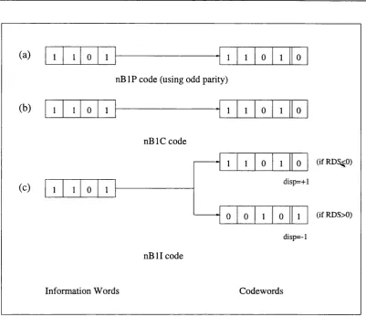
3.3.1 The n B lP , n B lC and n B l I line c o d e s ... 40
3.3.2 Improving the n B l I c o d e ... 42
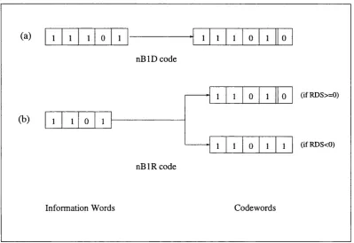
3.3.3 The n B lD and n B l R line codes ... 42
3.3.4 The n B lD R line c o d e ... 43
3.3.5 Improving the n B lD R c o d e ... 46
3.4 Summary of Code P e rfo rm a n c e ... 49
3.4.1 Decoding performance of the single added bit c o d e s ... 49
3.5 Spectral Properties of Selected n B l X c o d e s ... 52
3.6 Direct Calculation of the Power S p e c t r u m ... 53
3.6.1 Analysing the Manchester c o d e ... 55
3.6.2 Analysing the n B lD c o d e ... 56
3.6.3 Analysing the n B lC c o d e ... 58
3.7 S u m m a r y ... 58
4 S im u lation 63 4.1 In tro d u c tio n ... 63
4.2 A Communications System M o d e l... 65
4.2.1 Model c o m p o n e n ts ... 67
4.2.2 D ata source and e n c o d e r ... 68
4.2.3 Channel s im u la tio n ... 69
4.2.4 Hard decision d e c o d e r ... 72
4.3 Simulation Verification and V a l i d a t i o n ... 75
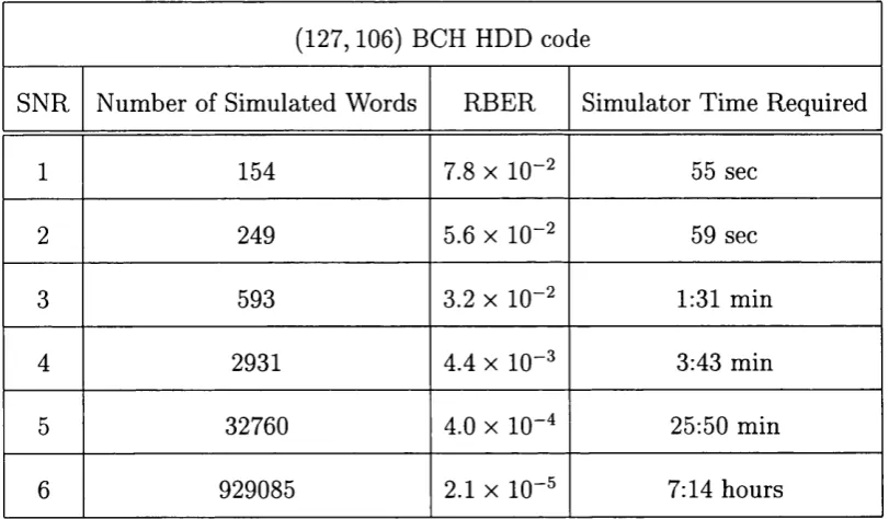
4.4 The Need for Accelerated Simulation Techniques... 77
4.5 Simulation Acceleration T e c h n iq u e s... 79
4.6 First Acceleration T e ch n iq u e... 79
4.7 Second Acceleration Technique ... 84
4.8 SDD and the Simulation Acceleration T e c h n iq u e s ... 88
4.9 O ther Performance Evaluation P r o g r a m s ... 89
4.9.1 Line code p e rfo rm a n c e ... 90
4.9.2 Power s p e c tru m ... 91
4.10 S u m m a r y ... 91
5 G en eralised C hase and th e A ID A lg o rith m 95 5.1 In tro d u c tio n ... 95
5.2 Generalised Chase A lg o rith m s ... 96
5.2.1 N c c selection and T P g e n e r a tio n ... 97
5.2.2 Simulation r e s u lts ... 102
5.2.3 Generalised Chase 3 ...105
5.3 Adaptive Immediate Decision A lg o r ith m ... 107
5.3.1 Description of the AID a l g o r ith m ...107
5.3.2 Threshold d e c i s i o n ...108
5.3.3 Optim al value of a ... I l l
5.3.5 Variable noise s im u la tio n s ... 116
5.4 Improving the Chase and AID A lg o r ith m s ...118
5.4.1 Decoding bounded alg o rith m ... 120
5.5 Summary ... 120
6 C om bining Error C ontrol and Line C oding w ith Soft D e c isio n D e cod in g 125 6.1 In tro d u c tio n ...125
6.2 The Need for Error Correcting Line C o d e s ...126
6.3 Generating E C L C s ...129
6.4 Proposed C o d e s ... 131
6.5 The n B l X Family of ECLCs ... 134
6.5.1 The n B l P E C L C ... 134
6.5.2 n B lC ^ n B lD and n B l R c o d e s ...138
6.6 Bi-modal E C L C s ... 139
6.7 Enhanced Flag P r o te c ti o n ...143
6.7.1 An example EFP c o d e ...145
6.8 CAB Algorithm D e s c rip tio n ...147
6.8.1 CAB N a lg o rith m ... 150
6.9 Simulation Results of the n B l X E C L C s ... 153
6.10 N= 2 E C L C s ...158
6.10.1 Improvements on the N=2 codes ... 161
6.10.2 Simulation results for the N=2 c o d e s ...163
6.10.3 Manchester ECLC ... 163
6.11 Calculating the Decoding Performance of the Single Flag Codes . . 171
6.12 Calculating the Decoding Performance of the EFP C o d e s ... 173
6.13 Rate Considerations ...176
6.13.1 Line code r a t e ... 179
6.14 S u m m a r y ... 182
7 C on clu sion s 186 7.1 C o n trib u tio n s ...187
7.2 Concluding R e m a r k s ...189
A C alcu latin g th e Pow er Sp ectru m 190 A .l In tro d u c tio n ...190
A.2 Calculating the Power Spectral D e n s ity ...190
A.2.1 Determining R y y { j ) at j = 0 191
A.2.2 Determining R y y { j ) at j 7^ 0 ...191
A .3 Power spectrum of the Manchester C o d e ...193
1.1 Coding tree diagram ... 3
2.1 Error correcting code tree diagram ... 13
2.2 Block diagram of a communications system ... 14
2.3 Communications system (with SDD) block diagram ... 22
2.4 Flow diagram of the Chase algorithm s... 24
3.1 AMI state diagram ... 37
3.2 AMI power spectrum ... 38
3.3 Examples of the P , C and I codes, for n = 4... 41
3.4 Examples of the D and R codes... 43
3.5 Flow diagram of the n B lD R code... 45
3.6 Worst case runlength for the 4 P 1 D P code... 48
3.7 Power spectrum for the n B lD code with n = 3... 53
3.8 Power spectrum for the n B lD R and n B l I codes... 54
3.9 Power Spectrum of the n B lD code with various values of n ... 57
3.10 Power Spectrum of the n B lC code with various values.of n ... 59
4.1 Communication system simulator outline... 66
4.2 Noise function shape... 72
4.3 Validation of (127,106) BCH code... 76
4.4 BCH (127,106) at SNR=5 simulated error distribution... 86
5.1 Simulation of a BCH (127,106) error correcting code with various values of TV... 104
5.2 AID algorithm flow diagram ...110
5.3 Performance comparison between the GC-2 and AID for a (127,106) BCH code, with sloping noise functions... 117
6.1 Conventional cascaded error correcting line code implementation. . 127
6.2 Error correcting line code block diagram ...129
6.3 Tree diagram of the presented ECLCs... 133
6.4 Percentage of code words with RDS values within ±1 versus code word length n...137
6.5 Power spectrum of a (7,3) ECLC...141
6.6 Cascaded added bit ECLC m atrix... 148
6.7 CAB flow diagram ... 149
6.8 Cascaded added bit ECLC with grouped (N = 2) code words...151
6.9 CAB ECLC rate gain for various group sizes, using a n = 127 BCH parent code with varying values of t ... 152
6.10 HDD performance using a parent BCH (7,4) ECC with and without ECLC properties... 155
6.11 SDD performance using a parent BCH (7,4) ECC with and without ECLC properties... 155
out ECLC properties... 156
6.13 Power spectrum of a (8,3) ECLC... 157
6.14 HDD performance of N=2 error correcting line coding code, using a (7.4) parent ECC...164
6.15 SDD performance of N=2 error correcting line coding code, using a (7.4) parent ECC...164
6.16 Block diagram of third algorithm... 166
6.17 Decoding performance of the third algorithm ...168
6.18 Spectral densities of the Manchester ECLC...170
6.19 CAB decoding performance for a (127,106) BCH code with SDD. . 174
6.20 Decoding performance for a (7,3) EFP ECLC...176
6.21 Rate comparison of similar codes... 178
6.22 ECLC rate comparison with n = 127... 181
6.23 ECLC rate comparison with n = 31... 181
List o f Tables
2.1 Linear block code with k = 4 information bits and n = 7 code word bits... 18
2.2 Number of T Ps for a n = 63 BCH code with various values of dmin
decoded using the Chase algorithms... 29
3.1 Encoding dictionary for the AMI code... 37
3.2 State table for the 3B 1D R code. The resultant disparity of each code word is shown in the brackets... 47
3.3 RDS bounds for the n B l X class of codes... 50 3.4 Maximum runlength characteristics of the n B l X class of codes. . . 51 4.1 Number of words and simulator time required for obtaining 1000
residual errors for varying SNRs... 78
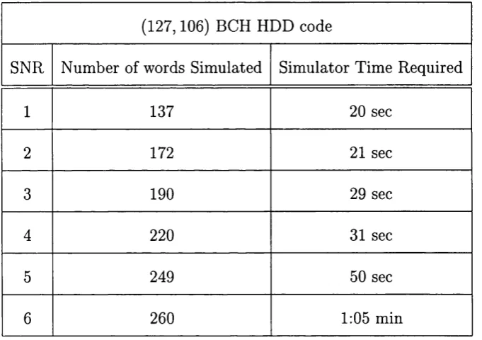
4.2 Simulator time required for obtaining 1000 residual errors at varying
SNRs using the first acceleration algorithm, compared with conven
tional simulation results... 83
4.3 Number of words and simulator time required for obtaining 1000
residual errors at varying SNRs... 87
5.2 Single error correcting performance using 2 T P s... 100
5.3 Single error correcting performance using 4 T P s... 101
5.4 Probability of incorrectly decoding a word for various numbers of
received errors...102
5.5 BCH (63,51) ECC at SNR=4 dB with various values of N (channel BER - 1.2 X 10⁻²)...106
5.6 BCH (127,106) ECC at SNR=5 dB with various values of N (channel
BER = 5.9 X 10⁻³)...106
5.7 Decoding performance versus average number of TPs for a (127,106)
BCH ECC code at SN R=4dB... 115 5.8 Decoding performance versus average number of TPs for a (63,51)
BCH ECC code at SNR=5dB... 115
5.9 Code performance simulation results...116
5.10 Number of times decoder is used for a BCH (127,106) ECC at a
SNR of 3 dB ...119
6.1 (8,4) Parity code words, together with their corresponding disparities. 136
6.2 Dictionary arrangement for a (7,3) BCH ECLC. The numbers in the
brackets indicate the disparity of each code word... 142
6.3 Runlength performance and rates of various ECLC codes...158
6.4 Comparison between rate and LC characteristics of various ECLC
C hapter 1
In trod u ction
1.1
Introduction
A m ajor aim of communication theory is to devise methods with which signals
can be transm itted though imperfect media with the highest possible degree of
reliability and efficiency.
In order to achieve this, the signal format at the transm itting end must be
chosen so th at it will offer maximum resistance to the channel impairments. Ad
ditionally, the receiver must be able to recover as much of the original signal as
possible. The application of coding is one method of achieving increased reliability.
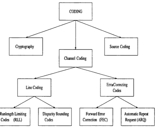
Generally, coding is a form of mapping whereby a given string of information
bits is converted into another sequence which j may have added redundancy. We
can divide coding into three major areas:
1. Source coding, which has two functions: [first to transform a message source
into a string of digital symbols and second, to remove any redundancy from
the word thus increasing efficiency.
2. Cryptographic coding, which is used to increase the security level of a sig
nal by concealing the message. This is done to ensure th a t only authorised
recipients can decode and obtain the transm itted information.
3. Finally, channel coding which aims to increase the reliability of a channel by
using added redundancy.
This thesis is concerned with channel coding, which can be further divided into
two main sub-areas:
1. Line coding (LC), in which the extra information is used to tailor the trans m itted signal in such a way as to match the characteristics of the communi
cations link.
Line coding can be used, for example, to modify the spectral characteristics
of the signal, (e.g. by placing constraints on the running digital sum (RDS)), or to place bounds on the runlength.
2. Error control coding, whereby extra bits introduced at the transm itter are
utilised at the receiver to detect and possibly correct any errors th a t may have
occurred. This is further sub-divided into automatic repeat request (ARQ) and forward error correction (EEC). Both ARQ and EEC will be examined in more detail in the next chapter.
C h ap ter 1 - Introduction
CODING
Source Coding
Disparity Bounding Codes
Forward Error Correction (FEC) Channel Coding
ErraCorrecting Codes Cryptography
Line Coding
Automatic Repeat Request (ARQ) Runlength Limiting
Codes (RLL)
Figure 1.1: Coding tree diagram.
Even though line and error control coding are two distinct operations they
both aim to increase the reliability of a system [1, 2, 3]. W ith the introduction of
digital systems in all aspects of modern life, the issue of data integrity is becoming
increasingly more im portant. Channel coding is a very attractive way of achieving
this.
This thesis concentrates on channel coding. A number of existing line and error
correcting codes will be presented and simulated, to identify their shortcomings.
In a number of cases, new codes will be introduced addressing these limitations.
The codes used will be very general in nature and simple to implement.
The basic concepts behind channel coding are initially presented. These are
then used to build more complex line and error control codes. However, it is not
uncommon for a designer to incorporate both aspects of channel coding in a system.
at the decoder. It will be shown th at this cascaded scheme can be inefficient
and reduces the overall decoding performance. For these reasons combined error correcting line codes (ECLCs) have been devised which offer improved performance [4, 5],
Finally, the concept of soft decision decoding (SDD) will also be introduced. This is a technique which combines the demodulation and decoding processes. A
number of the codes presented in this thesis can be improved by the use of SDD.
The latter increases the complexity of the receiver but offers increased decoding
power without adding extra redundancy.
A particular feature of the thesis is an exploration of the benefits th a t arise
from employing SDD with ECLCs. This enables significant improvements in both
rate and decoding power to be realised. There is currently considerable interest in
channel coding for high bit rate systems, such as undersea optical telecommunica
tions transmissions, which provided the original motivation for this study. For this
reason only low complexity codes (which allow high bit rates to be realised) will
be considered.
1.2
T hesis Organisation
The structure of this thesis can be briefly summarised as follows;
Following this introduction, chapter 2 contains the fundamentals of error control
coding together with examples of various simple codes. This chapter is used as
a basis for the introduction and development of more advanced codes which are
C h ap ter 1 - Introduction
are extensively examined due to their critical role in the following chapters, and
especially in chapter 5.
Chapter 3 presents the basics of line coding together with a family of simple
‘added b it’ codes. These offer tight runlength and disparity bounds while being
very simple to implement. A number of the added bit codes are used in chapter 6
to form error correcting line codes.
In chapter 4, the need for simulation in channel coding is presented together
with a basic ECC simulation. The latter is used as a basis for developing two
new simulation acceleration algorithms which are used throughout the thesis to
validate theoretical results. These work by ‘eliminating’ a large number of code
words without affecting the accuracy of the simulation.
Chapter 5 introduces three novel SDD algorithms which offer significant perfor
mance improvements. Specifically, the generalised Chase (GC) utilises an increased number of test ^atterns^o achieve improved decoding performance; the AID algo rithm then uses threshold decoding to reduce the average number of test patterns
without affecting the decoding performance. Finally, the T P E algorithm reduces
the number of test patters required for SDD, by eliminating those th a t produce
the same estimated error pattern (EEP).
In chapter 6, existing concatenated and ECLCs are presented together with the
reason behind the need for error correcting line codes. These are used as a basis for
the generation of novel codes, which also utilise SDD to provide better performance
with minimal increase in complexity.
mendations for future work.
1.3
Sum m ary o f M ain C ontributions
The research presented in this thesis examines channel coding schemes suitable for
high bit rate systems. The major contributions fall into four main interlinked areas
and can be summarised as follows:
• New line codes: a new family of ‘added b it’ line codes was introduced, which
resulted in the harmonisation into a single identifiable family of the disparate
n B l X codes.
• Improved simulation techniques, where two novel simulation acceleration
techniques are developed. These significantly reduce the amount of time
required for obtaining statistically accurate results without compromising
accuracy.
• Novel SDD algorithms: a number of novel SDD algorithms are introduced
which offer improved decoding performance and increased decoding speed
without significantly increasing the complexity of the decoder.
• New error correcting line codes: SDD was combined with conventional error
correcting line codes thus producing novel codes which can offer both accept
able decoding performance and reasonably good line coding characteristics.
C hapter 1 - Introduction
1. Y . Bian, J. O ’Reilly, A. Popplewell, S. Fragiacomo: “New Simulation Tech niques for Evaluation Telecommunications Transmission Systems with FEC” ,
Fifth lE E Conference on Telecommunications, March 1995, UK.
2. S. Fragiacomo, Y. Bian, A. Popplewell, J. O ’Reilly: “A New Low Complex
ity Near ML Soft Decision Decoding Algorithm for Linear Block Codes” ,
lE E Singapore International Conference on Communication Systems, IEEE ICCS/ISPACS ’96, 25-29 November 1996, Singapore.
3. Y. Bian, A. Popplewell, J. O ’Reilly, S. Fragiacomo, R. Blake: “FEC for
Future Trans-Oceanic Optical Systems” , Fifth lE E Conference on Telecom munications, Brighton, March 1995, UK.
4. S. Fragiacomo, C. Matrakidis, J. O ’Reilly: “Exploiting Soft Decision Decod
ing for Error Correcting Line Codes” , lE E Singapore International Confer ence on Communication Systems, IEEE ICCS/ISPACS ’96, 25-29 November 1996, Singapore.
5. S. Fragiacomo, C. Matrakidis, J. O ’Reilly: “A Novel Error Correcting Line
Code” , Third Communication Networks Symposium, 8-9 July 1996, Manch ester, UK.
6. S. Fragiacomo, C. Matrakidis, J. O ’Reilly: “A New Error Correcting Line
Code” , IT S /IE E E ROC&C ’96 International Telecommunications Sympo sium, October 28-31 1996, Acapulco, Mexico.
7. S. Fragiacomo, C. Matrakidis, J. O ’Reilly: “A Novel Error Correcting Line
Ses-sion, June 25-28 1996, Heidelberg, Germany.
8. S. Fragiacomo, C. Matrakidis, J. O ’Reilly: “Soft Decision Error Correcting
Line Code for Optical D ata Storage” , 9th Annual Meeting, LEO S 96, 18-21 November 1996, Boston, USA.
9. S. Fragiacomo, C. Matrakidis, A. Popplewell, Y. Bian, J. O ’Reilly: “An
Accelerated Simulation Technique for Evaluating Communication Systems
Utilising FEC” , Networks and Optical Communications (NOC), June 17-20 1997, Antwerp, Belgium.
10. S. Fragiacomo, C. Matrakidis, J. O ’Reilly: “A Class of Low Complexity Line
Codes” , International Symposium on Information Theory, IS IT 91, 29 June 1997, Ulm, Germany.
11. S. Fragiacomo, C. Matrakidis, J. O ’Reilly: “Performance Aspects of a Class of
Low Complexity Line Codes” , International Conference on Signal Processing, IC SP A T 97, September 1997, San Diego, USA.
In addition, a number of journal papers have been submitted. The next chapter
begins by presenting some basic concepts of error control coding and soft decision
B ibliography
[1] K. W. Cattermole: “Mathematical Foundations for Communication Engineer
ing” , Volume 2, Pentech Press, 1986.
[2] S. Lin, D. Costello: “Error Control Coding” , Prentice Hall, 1983.
[3] “Algebraic Coding Theory and Applications” , Edited by G. Longo, Springer-
Verlag.
[4] A. Popplewell: “Combined Line and Error Control Coding” , PhD Thesis, University of Wales, Bangor, 1990.
C hannel C oding
2.1
Introduction
In this chapter a brief overview of forward error control (FEC) and soft decision decoding (SDD) will be presented. As discussed before, channel coding can be di vided into two main categories: FEC and line coding (LC). This chapter introduces the basic concepts behind FEC, while chapter 3 presents the basic concepts of line
coding.
2.2
Error Control Codes
In general, error control codes can be divided into two types [1]:
1. Automatic repeat request (ARQ), whereby the receiver can only detect errors. If these occur, then a feedback path is used to request the re-transmission
of the erroneous data. ARQ systems can be divided into two m ain cate
gories: stop-and-wait ARQ and continuous ARQ. W ith stop-and-wait ARQ
C hapter 2 - Forward Error Control 11 the transm itter will only send the next word if the received word contains
no errors. Continuous ARQ will send words and receive acknowledgements
continuously, jf errors are detected the offending code word will be re
transm itted. ARQ systems can be simple to implement since they only
require error detecting codes and are efficient in high signal to noise ratio
(SNR) communication links. However, a number of disadvantages are also
present:
• They require a feedback path to send the repeat request. This means
th a t stop-and-wait ARQ requires a half-duplex channel while continuous
ARQ requires a full-duplex channel.
• They can be very inefficient, especially if high channel error rates exist
because a high number of repeat requests will be made.
• In high bit rate or long distance systems where a significant delay exists,
continuous ARQ will be used. This can be more efficient but will require
large buffering systems.
For the above reasons ARQ systems are not considered here.
2. The second error control strategy is forward error correction (FEC). This utilises codes which can detect and correct errors at the receiver, termed error correcting codes (ECCs). Such codes are more complicated to implement but do not require feedback paths. In addition, they are better suited to relatively
low SNR applications. For these reasons, FEC is examined in more detail in
2.2.1
Forward error correction
The theoretical basis for error correcting codes was developed during the late 1940’s
by Shannon [2]. He suggested th at the elimination of errors in a received digital bit
stream was possible, if the latter was properly encoded. Encoding usually requires
the introduction of redundancy. Shannon also proved th a t any number of errors
can be corrected, provided the block length is large enough.
The challenge in coding theory is to discover codes which can correct a large
number of errors while minimising redundancy and complexity.
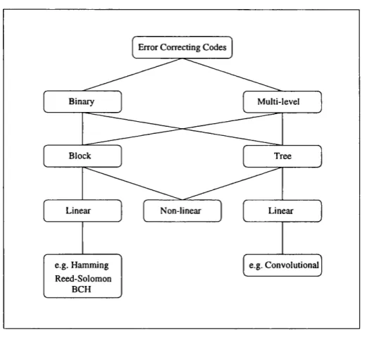
Error correcting codes can be divided into binary and multi-level codes. If the
encoded data stream at the transm itter can only obtain two distinct values then
our code is a binary one, otherwise it is a multilevel one. Both these types of code
can be further sub-divided into block or tree codes. Block codes, which are of
interest here, were introduced by Hamming in the 1950’s [3]. They differ from tree
codes in th a t there is no ‘memory’ during the encoding process and the produced
bits depend only on the current information word.
Finally, either of these codes can be linear or non-linear. A binary block code
is linear if the modulo-2 sum of any two of its code words is also a code word. The
best known linear block codes are cyclic, where a cyclic shift of any code word also
produces a code word. The most frequently used ones are the BCH codes which
include the Reed-Solomon and Hamming families. The most common tree codes
are convolutional codes, where the check bits are mixed with the information bits
in a continuous manner.
C h ap ter 2 - Forward Error Control 13
Error Correcting Codes
Binary Multi-level
Block Tree
Linear Non-linear
e.g. Hamming Reed-Solomon
BCH
e.g. Convolutional
Figure 2.1: Error correcting code tree diagram.
This thesis aims to develop error correcting and line codes appropriate for mod
ern high bit rate systems. For this reason, only linear binary block codes will be
considered as they are likely to be the simplest to implement and usually require
a minimal amount of decoding time. A widely used group of such codes are the
Bose-Chaudhuri-Hocqenghem (BCH) codes, introduced in 1960 [4]. These will be used as an example whenever a specific code example is required.
2.3
G enerating Linear Binary Block C odes
Figure 2.2 is intended to make linear block error correcting codes easier to appre
ciate. This represents the block diagram of a complete communications system,
utilising an (n, k) ECC encoder.
The digital data source will generate a continuous stream of information bits.
Digital D ata
Source u=(u ,u ...u ECC Encoder v=(v ,v ...V M odulator
Noise and Interference
TX system
n co dcw tird trils
ECC Decoder D em odulator
D ata D estination
Figure 2.2: Block diagram of a communications system.
These are represented by a binary k —tuple Ti = {uq, ... , Uk_i) called a message.
This implies that for a binary code there are 2^ possible messages.
The encoder ‘contains’ the generator matrix G which has as rows a set of k
linearly independent code words. These are called the ‘basis code words’ and make the row space of G the linear code. If all the linear combinations of the basis code words are taken {v = ü ■ G) then 2^ n-bit code words will be generated.
The error correcting capabilities of a code depend on the Hamming distance (d) separating the code words. The Hamming distance of two code words of length n
C h ap ter 2 - Forward Error Control 15 termed the ‘error correcting capability’ of the code.
At the output of the encoder the k-hit information vector will therefore be transformed to an n-bit code word which now has error correcting properties. The
added (n — k) bits are called the parity check digits, or parity bits. The n-bit code word is then m odulated and transm itted. The same process is repeated for the
next k information bits. An (n, k) code of minimum distance {dmm) has therefore been generated.
At the receiver, the received waveform is initially demodulated. This produces
a binary stream of code words. If no errors have occurred then the received vector
f will equal the transm itted one, i.e. f = v. If errors have occurred, then it can be assumed th a t they will have formed the error vector ë. In such a case f = ü 0 ë,
where 0 indicates modulo-2 addition.
It is up to the decoder to attem pt to detect and possibly correct the errors
th a t may have occurred. To do this it uses the parity check m atrix H. This is a
{{n — k) X n) m atrix where any vector in the row space of G is orthogonal to the rows of H. Therefore, for any v we get v • = 0, where is the transpose of H.
In order to detect if errors have occurred, f is multiplied by If f • = 0 then either no errors have occurred, or the error correcting capability (t) of the code has been exceeded.
If error correction (as opposed to error detection) is also required, then the
previous formula must be expanded. At the receiver f is multiplied by i.e.
f = = v - H ^ F
product is called the syndrome (S) and only depends on the error pattern. If the syndrome is zero then no errors have occurred; unique syndromes exist, each
corresponding to a specific error vector. Using the syndrome information the error
position can be located. Since our codes are binary there are only two possible
distinct bit states, a logic 1 or a logic 0. Therefore if the positions of the errors in
the code word are known, error correction is also possible by performing a simple
inversion of those positions.
2.3.1
A sim ple ECC exam ple
To provide an illustrative framework for some basic definitions, an example of a
very simple linear binary (7,4) code with a minimum Hamming distance dmin = 3 will be considered. This has k = A information bits encoded into n = 7 code word bits. Therefore, 2^ possible distinct messages will be encoded into 2” code words
using a one-to-one correspondence. The generator m atrix G of such a code is of the following form:
G =
^0
9i
92
9z
1 1 0 1 0 0 0
0 1 1 0 1 0 0
1 1 1 0 0 1 0
1 0 1 0 0 0 1
while the parity check m atrix H will be the following
C h ap ter 2 - Forward Error Control 17
H =
1 0 0 1 0 1 1
0 1 0 1 1 1 0 (2.2)
0 0 1 0 1 1 1
Assume th a t a message ü = (1101) must be transm itted using the above code. To achieve this, the message must be multiplied with the generator m atrix so th at
the code word vector v is produced, i.e.
V = Ü ' G = (1101) C — 1 - po 4-1 ' T 0 - ^2 T 1 ' p3 —
( 1101000) + (0110100) + (1010001) = 0001101
Thus the transm itted EC code word will be 0001101. Because the (7,4) code
is a systematic one, the four last bits contain the original message in the correct
order, while the initial three bits are the parity bits required for error detection
and correction at the receiver. Table 2.1 contains the mappings for all possible four
bit information words.
2.4
D ecoding a Sim ple ECC
In the previous section, a 4-bit information message was encoded into a 7-bit code
word using a linear block code. In this section, the received word will be decoded
and up to t errors will be corrected. Since t = and for our code dmin = 3 then t = 1, i.e. it is a single error correcting code.
Assume th a t f = (ro, r i , r 2, rs, r 4,rs, re) is the received vector. The syndrome
Information word (7,4) code words
0000 000 0000
0001 101 0001
0010 Oil 0010
0011 010 0011
0100 o i l 0100
0101 110 0101
0110 010 0110
0111 001 0111
1000 110 1000
1001 o i l 1001
1010 001 1010
1011 100 1011
1100 101 1100
1101 000 1101
1110 010 1110
n i l 111 n i l
C h ap ter 2 - Forward Error Control 19
S = s = r ' = (so, Si, ... , S(„_fc_i)). (2.3) From this it is deduced th a t the syndrome is simply the sum of the received
parity digits and those re-computed at the decoder. Thus if 5 / 0 an error has
been detected.
Using equation 2.3 in our example (7,4) code the following equation is obtained;
s = (sq, Si, S2) = f ’ = {u F ë) - = ü • + ë - = 0 F ë ’ = ë • Assuming th a t the vector f = (1001001) has been received, i.e. a single error exists in bit position 5 the syndrome will be equal to:
5 = f • 77^ - (1001001)
100
010
001
110 Oil 111 101
= (111) (2.4)
Therefore S ^ 0 and an error has been detected. In order to detect the error position it is noted th at
(111) — (co, ei, 62, 63,64,65, eg)
100
010
001
110 Oil 111
101
(2.5)
Using equations 2.4 and 2.5 the following error vectors are derived:
1 — 60 + 63 + 65 + 66
1 — 6 1 + 6 3 + 6 4 + 6 5 1 — 6 2 + 6 4 + 6 5 + 6 6
(2.6)
(2.7)
(2 .8)
A number of possible solutions exist th at satisfy the above equations. If max
imum likelihood decoding is used for error location then the error pattern with
the minimum number of corrected positions is selected. In this case, this is the
(0000010) error vector. If this is added to our received vector the transm itted
vector will be obtained.
In chapter 4, Berlekamp’s iterative algorithm will be briefly presented. This
is an algorithm for generating the error locator polynomial, appropriate for more
complex and powerful codes. It is a well-established technique which lends itself
C hap ter 2 - Forward Error Control 21
2.5
Soft D ecision D ecoding
In the previous sections it was dem onstrated how the information bits could be
encoded and decoded so th at error detection and correction were possible. At
the receiver, only the algebraic properties of the code were utilised to locate any
possible errors. This is termed hard decision decoding (HDD).
In this section, the basic principles of soft decision decoding (SDD) are pre sented. SDD uses the analogue information to try to increase the error correcting
capability of the code. As has been mentioned before, a code of minimum distance
dmin can correct up to t errors. The use of SDD allows this limit to be exceeded, under certain conditions. The penalty is the increased complexity of the decoder
and the fact th at the t-error correcting capability ^ ^ 7 not be guaranteed anymore
SDD techniques are not suitable for very noisy systems. However, modern telecommunication and data storage systems usually have very low error rates and
can thus benefit from the application of such techniques.
A modified communications system which includes SDD, is shown in figure 2.3.
Here extra information is provided to the decoder in the form of the analogue
values of the received bits. These values are provided by the demodulator and are
used to facilitate the decoding process by indicating possible error positions.
SDD algorithms can be grouped into two broad classes:
(a) Minimum distance (or minimised sequence error rate) decoding algorithms,
based on [6].
(b) Trellis decoding algorithms, adapted for block codes.
Digilal Data
ECC Encoder M odulator
u=(u ,u ...u v = ( v ,v V
(k-1)
N oise and Interference
TX system
ECC Decoder Dem odulator
Analogue Infotm ation
Figure 2.3: Communications system (with SDD) block diagram.
used are the Chase algorithms. This is because they can offer a balance between
decoding power and complexity. In the following sections the Chase algorithms will
be examined in detail. Their shortcomings will be identified and then addressed in
chapter 5.
2.5.1
T he Chase algorithm s
In 1972, D. Chase [7] suggested three different SDD algorithms of type (a), each
of which provided a different number of test patterns, allowing a trade-off between
performance and complexity. Specifically, the Chase decoder generates a set of
possible error patterns, called the test patterns (TPs). These are then sequentially perturbed with the received word and taken through a conventional HDD decoder.
C hapter 2 - Forward Error Control 23
error pattern (EEP). The EEP is used to indicate the bit positions which are deemed to contain an error and each is assigned a confidence value, provided by
the analogue information. After HDD of all possible patterns has taken place, the
one with the highest confidence value is selected and added to the received word
to provide the corrected word.
Chase suggested three different algorithms, each examining a different number
of TPs. The TPs are used to invert a number N of least confidence bit (LCB) positions. These are defined as the bit positions closest to the decision threshold.
The reason behind the use of TPs is th at if the voltage value of a received bit is
very close to the decision threshold, this bit is very likely to be in error. Thus
if the syndrome calculations indicate th at the received code word contains errors,
these are more likely to be in the LCB positions than anywhere else. By systematic
inversion of different combinations of these positions, the errors within a code word
could be corrected.
An ECC utilising HDD can correct upto errors. The use of an SDD
algorithm, in conjunction with an ECC, allows a higher average number of errors
per code word to be corrected. However, unlike a conventional ECC, the use of any
SDD algorithm may not guarantee the correction of up to t errors within a code word.
The flow diagram of the decoding process for the Chase algorithms is shown in
NO Is an EEP
possible ?
YES
NO
YES
NO
YES Have any EEPs heen generate(^ ^H av e all TPs^ heen generatec^
Accept received word Find analog weight and store.
Add TP to received word HD decode
Select EEP of lowest analogue weight Add it to the received word and decode
Receive word Generate LCB table
Generate TPs according to LCB table
C hapter 2 - Forward Error Control 25
2.5.2
M echanics o f th e Chase algorithm s
Assume th a t for a given communication system the transm itted word is defined as
V = Vq, ui, ... U(n-i) and the received word a sr = Tq, ri, ... where = Vi-\-n0i for 0 < z < (n — 1) and noi is defined as the noise amplitude. Let t be the error correcting capability of the (n, k) ECC.
The resultant error pattern (EP) indicates the bit positions where v and r
differ, ë = eo,ei, ... e^-i is termed the error vector and is defined by = u* 0 for 0 < z < (n — 1) while the binary weight of ë is termed W{e) and defined as the total number of non-zero elements in the sequence. A decoder will try to find
a code word th a t satisfies W{e) < where dmin is the minimum Hamming distance of the code.
In the Chase algorithms, a test pattern T P = tpo,tpi, ... tp(n-i) for 0 < z < (n —1) of length n is initially generated. This is done by selecting a number (Nchase)
of LCBs and producing a set of n-bit sequences containing possible perm utations
of these Nchase positions. This generates a set of upto TPs. The initial TP will always be the all zero word.
Each TP is then modulo-2 added to the received word f and the resultant
sequence f ' = r 0 T P is conventionally decoded using any suitable HD decoder.
Since the addition of the TPs has the effect of inverting a number of LCB positions
it is likely th a t some of the resultant sequences will have a reduced number of errors
compared to the received code word.
If a conventional HD error correcting decoder was used and the initial number
the T P procedure, it is possible th at the total number of errors is reduced (or even
eliminated) thus allowing conventional decoding to take place.
The received word with the added T P will be taken through the EC decoder,
which will either produce a decoder error pattern (DEP) or fail to decode. The DEP will then be added to the T P to produce an n —bit sequence termed estimated error pattern. Thus, E E P = (eepo.eepi, ... eep^n-i)) = T P 0 D E P . If the addition of the T P has introduced more errors (instead of eliminating them) it is possible th at
the decoding will fail. In such a case no EEP will be produced. This is the reason
for always starting with the all zero word as the initial TP; if the error pattern
contains t or less errors the all zero TP will allow the decoder to operate properly. If not, then only the removal of errors will allow decoding. The latter can only be
accomplished by using appropriate TPs and for this reason the process is repeated
for the whole T P set.
Once all possible EEPs have been produced, one must be selected. It should
be noted th at not every TP will create an EEP and not all EEPs will be distinct.
The selection will be done using the analogue weight of each EEP which is defined
as;
n — 1
aw EEP = ^ «2 X eepi (2.9)
2 = 0
where 0% is the analogue value of the i — th bit position of the EEP.
The EEP with the smallest analogue weight will be modulo-2 added to the
received word and the resulting sequence will be accepted as the corrected word.
C hapter 2 - Forward Error Control 27 the pattern which has inverted the least confident bits. If all errors have been
corrected then the EEP should equal the EP.
2.5.3
Test p attern set generation
It should be clear th a t the generation of the T P set is a very im portant task. If
this is correctly generated then the total number of errors in a code word may be
reduced, otherwise it will be increased. For this reason, the introduction of channel
measurements may not guarantee anymore the correction of a minimum number of t received errors. However, if the total number of errors is above t, the decoder may have the ability to correct them. The three algorithms for selecting the TPs
as suggested by Chase are the following:
1. The first algorithm (Chase 1) examines all possible TPs. Therefore, for an
n-bit code with a minimum distance between code words of dmin, a total of (, i) possible combinations exist. For other than very small values of n
L 2 J
this is impractical to implement in hardware or indeed to simulate down to
the RBERs of interest. A considerable reduction in complexity is obtained if
the test patterns th a t produce identical error patterns are ignored, but even
with this improvement, the algorithm is not very efficient.
2. The second algorithm (Chase 2) considers only the set of error patterns con
taining Nchase = lowest channel measurements (i.e. the bits with the highest probability of error). The test patterns generated in this case are
those where any combination of inverted positions is allowed within the set
3. Chase 3 examines Nchase = ( [ ^ ^ J + 1) possible patterns. Once more the inverted positions are assigned to the i positions of lowest confidence. If
dmin is even, i takes the values i = (0,1,3, ... d — 1). If dmin is odd then
i = (0,2,4, ... d — 1). This algorithm gives best results for codes with large values of
dmin-Chase does not give the reason for differentiating between odd and even
values of dmin and work done on the simulator indicates th a t it is unnec essary. Specifically, the performance of a code decoded using Chase 3 with
z = (0,2,4, ... d — 1) never exceeds the performance of the same code using Chase 3 but with ? = (0 ,1,3, 5, ... d ~ 1).
2.5.4
Perform ance com parison o f th e C hase algorithm s
Each of the three Chase algorithms utilises a different sized set of T Ps for decoding.
Clearly, if the TPs are sensibly chosen, the larger the set of TPs the more decoding
power the code will have. However a large set of TPs will require more tim e to
decode since a decoding operation for each TP is required.
Clearly, for large n (even for a relatively small dmin) algorithm 1 is too complex to employ in practice, since it will examine (,2,) possible error patterns. The second
L 2 J
Chase algorithm will examine 2^1-f J) possible error patterns. Finally, using the third
Chase algorithm ( [ |J - I - 1) possible test error patterns must be examined.
The above figures indicate th at the complexity of Chase 2 and 3 depends on
C h ap ter 2 - Forward Error Control 29 in table 2.2 where the to tal number of TPs needed for each Chase algorithm are
shown for various values of dmin, for an n = 63 BCH code.
t Chase 1 Chase 2 Chase 3
1 63 2 2
2 1953 4 3
3 39711 8 4
4 595665 16 5
5 7028847 32 6
Table 2.2: Number of T Ps for a n = 63 BCH code with various values of dmin
decoded using the Chase algorithms.
In terms of decoding power, Chase 1 will provide results which will closely ap
proach the maximum likelihood (ML) limit. The latter is the best possible decoding result soft decision decoding can offer. Simulation results indicate th at Chase 2
performs reasonably well when compared to Chase 1, particularly at the low error
rates of importance for this study. A significant reduction in the number of T Ps is
effected while an acceptable decoding performance is maintained. Chase 3 involves
a loss in performance compared to the second algorithm due to the reduced number
of TPs.
A disadvantage of all 3 algorithms is the fact th a t the complete set of T Ps needs
to be generated and used before one can be selected. This can prove to be too time
2.6
Sum m ary
In this chapter, the basic definitions and concepts of error control coding (which
included both hard and soft-decision decoding algorithms) were introduced. The
Chase SDD algorithms were then described in detail and a critical assessment of
their performance was made. Thus the second Chase algorithm was found to be
the most promising choice for implementation in practical high rate systems. This
is because it offers a balanced solution in terms of decoding power and simplicity.
The latter is very im portant both because it allows improvements to be made and
also because of the potential application on high bit rate systems.
Having introduced some key ideas relating to error correcting codes we now turn
our attention in the following chapter to line coding. We will begin by reviewing the
basic principles and then progress to the consideration of some novel low-complexity
B ibliography
[1] S. Lin, D. Costello: “Error Control Coding” , Prentice Hall, 1983.
[2] C. Shannon: “The M athematical Theory of Communication” , Bell Systems Technology Journal, 1948.
[3] R.W. Hamming: “Error detecting and Correcting Codes” , Bell Systems Tech nology Journal, Vol. 29, pp. 147-160, April 1950.
[4] R. Bose, D. Ray-Chaudhuri: “On a Class of Error Correcting Binary Group
Codes” , Information and Control , Vol 3, March 1960. [5] The Open University: “Codes” , TM 361 14, 1982.
[6] G. D. Forney,“Generalised Minimum Distance Decoding” , IEE E Transactions on Information Theory, Vol IT-12, pp. 125-131, April 1966.
[7] D. Chase: “A Class of Algorithms for Decoding Block Codes W ith Channel
Measurement Information” , IEEE Transactions On Information Theory, Vol IT-18, pp. 167-170, January 1972.
[8] O. Olanyian: “Implementable Soft-Decision Decoding Schemes” , International Journal Of Electronics, Vol 66, 1989.
[9] J. Eiguren, I. Burner, P. Farrell: “Split Syndrome Soft-Decision Decoding For
Block Codes” , Coding and Cryptography Conference, December 1993.
[10] J. Wolf: “Efficient Maximum Likelihood Decoding Of Linear Block Codes
Using a Trellis” , IE E E Transactions On Information Theory, Vol 24, January 1978', pp. 76-80.
[11] W. H. Thesling, F. Xiong: “Pragm atic Approach to Soft decision Decoding
C hapter 3
Line C oding
3.1
Introduction
In the previous chapter, the basic concepts of forward error correction (FEC) were presented. Soft decision decoding (SDD) was then introduced which offered greater
error correcting (EC) capabilities but at the expense of increased complexity. A number of existing SDD algorithms were presented and critically evaluated.
In this chapter, line coding (LC) will be introduced. Specifically, the need for LC will be presented together with some basic definitions and concepts. Those will
be followed by the presentation of a new family of line codes which are very simple
to implement, yet offer reasonably tight bounds for both the maximum runlength
and the disparity. Since they are single added bit codes, the overall rate is not
significantly reduced which makes them well suited to high bit rate applications.
The chapter begins with a presentation of the basics of line coding, a simple
line code being used as an example to illustrate the main concepts. The n B l X
family of line codes is then introduced followed by a detailed examination of its
performance. We conclude by presenting two methods for determining the power
spectrum of a line code.
3.2
Line Coding
The principal function of a line code is to match the transmission signal to the
communication channel characteristics. Therefore, line coding is introduced to
overcome the physical impairments of the channel used. This is usually achieved
by limiting or eliminating the low frequency content of a signal an d /o r by reducing
the maximum runlength. Both of these factors require added redundancy.
The low frequency content must be restricted since most channels cannot achieve
sufficient signal to noise ratio in th at area of the spectrum [1]. For example, mag
netic recorders do not respond well to low frequency signals, so th a t a signal th at
contains such components will have an increased number of errors. These can be
corrected by using EEC. However, a simpler technique is to code the d ata so th at
distortion is minimised. This can be achieved by line coding [2].
In addition, for practical reasons, many channels are AC coupled. This implies
th a t the DC and low-frequency content of a signal must be suppressed [3, 4]. This
can be achieved by bounding the digital sum variation (DSV), which is the differ ence between the largest and smallest values of the running digital sum (RDS) [5], defined as
C hapter 3 - Line Coding 35 where di is defined as the disparity (i.e. the difference in ones and zeros) of each one of the k code words.
Additionally, it is common for the receiver to be synchronised by extracting
timing information from the received waveform. It is thus necessary to have an
adequate number of transitions within a given amount of time. This is achieved by
limiting the maximum runlength (RLmax) of a bit stream. The latter is defined as the maximum number of consecutive identical bits in a code word.
Recent experimental data suggest th at significant gains in error performance
can be achieved in some systems by limiting the maximum runlength of a trans
m itted word. Specifically, in a 232km optical fibre system, AdB of equivalent coding gain was present simply by limiting the maximum runlength from RLmax = 31 to
RLmax = 7 [6].
Generally speaking, a line code will map a block of k symbols which have p
levels into a block of m symbols with r levels. In most cases the use of the line code will introduce some redundancy, so th at The rate R of a code is
defined as
D _ k l o g 2 P m l o Q 2 r '
A disadvantage of most line codes is known as ‘error extension’. This is a
phenomenon whereby errors along the channel give rise to a larger number of errors
in the decoder. An example of error extension will be presented in the following
sections with the introduction of the bi-modal codes.
The following evaluation factors can be used to compare various line coding
1. Power Spectrum: This usually is one of the most im portant factors, indicating
the extent of any DC or low frequency contents. The low frequency region of
the power spectrum is related to the running digital sum bounds.
2. Synchronisation: In most applications, the receiver utilises signal transitions
to synchronise itself with the transm itter so th at optimal sampling is effected.
Therefore, a code which offers a high number of transitions is preferred. Syn
chronisation is determined by the maximum runlength.
3. Signal degradation: Very frequent transitions can in some instances (e.g.
bandw idth limited channel) cause inter-symbol interference (ISI) between ad jacent symbols.
4. Reduction in the overall bit rate R, due to the introduction of the line code. 5. Complexity of implementation and cost.
Various existing and new line codes will be presented in this chapter with the
areas mentioned above forming a basis for assessing their suitability for use.
3.2.1
A sim ple line code
One of the simplest line codes is the alternate mark inversion (AMI) code. Such a code is not very useful for optical transmission systems since the three transition
levels required are not suited to on-off keying techniques. However, AMI will be
used to dem onstrate, by way of example, the basic concepts behind line coding.
C h ap ter 3 - Line Coding 37 alternately. Thus long runs of ones will be avoided while long runs of zeros can
still exist. The encoding dictionary for this code is shown in table 3.1.
Information Word Code word
RDS=0 RDS=1
0 0 0
1 +1 -1
Table 3.1: Encoding dictionary for the AMI code.
Figure 3.1 presents the state diagram of the AMI code. A state diagram is a
convenient way of showing the possible states a code can have (represented by a
circle) and the probability of transferring from one state to another. Figure 3.1
indicates th a t in the AMI code there is an equal probability of transferring between
different states or remaining in the same state. 0.5
0.5 0.5
R D S=1 R D S= 0
0.5
Figure 3.1: AMI state diagram.
Finally, the power spectrum of a line code is very im portant. As has been
mentioned before, one of the reasons behind the use of a line code is the suppression
spectrum presents the power spectral density versus frequency for a given code. In
our case this was achieved by using the Cariolaro and Tronca algorithm [7]. The
power spectrum of the AMI code is illustrated in figure 3.2, where it is seen th at
indeed the lower frequencies are suppressed and the DC content is zero.
2 .5
Q
Q . CO
Q_
0 .5
0.8 0 .9
0.1 0.2 0 .3 0 .4 0 .5
N orm alised freq u en cy 0.6 freq u en cy
0 .7
Figure 3.2: AMI power spectrum.
In the following sections a unified family of line codes, termed n B l X , is exam ined. This is simple to implement and can offer very good line coding characteris
tics.
3.3
The
n B l X
Class o f Line C odes
C hapter 3 - Line Coding 39 word bits. A widely used subset of these codes are those where m = (n + 1), i.e. a single bit has been added to every n information bit block. The added bit can be used to achieve either error detection or line coding properties. The n B l X
line codes introduced here are a subclass of this family [4, 8, 10]. These are very
simple to implement and relatively effective but, like all line codes, they reduce
the overall code rate, which becomes equal to R = { ^ ) = ( ^ ^ ) , and under certain circumstances, may introduce error extension.
The major advantages of the n B l X codes can be summarised as follows: • They can provide tight runlength and disparity bounds.
• The reduction in rate (especially for large values of n) is minimal. • They can be very simple to encode and decode.
• They use state-independent decoding. This means th a t the decoder does not
utilise the RDS information so error propagation between line code words is
impossible.
• Finally, most added bit line codes can be converted into error correcting line codes (ECLCs).
This chapter introduces a number of novel single added bit codes. These are
combined with existing line codes, to form the n B l X family. Each member of this family is presented in detail, together with any possible improvements, in the