Automatic height extraction from stereoscopic SAR imagery

AUTOMATIC HEIGHT EXTRACTION FROM

STEREOSCOPIC SAR IMAGERY

A Thesis subm itted for the degree of

Doctor of Philosophy

in the U niversity o f London by

Zway-Gen Twu

All rights reserved

INFORMATION TO ALL USERS

The quality of this reproduction is dependent upon the quality of the copy submitted.

In the unlikely event that the author did not send a complete manuscript and there are missing pages, these will be noted. Also, if material had to be removed,

a note will indicate the deletion.

uest.

ProQuest 10046027

Published by ProQuest LLC(2016). Copyright of the Dissertation is held by the Author.

All rights reserved.

This work is protected against unauthorized copying under Title 17, United States Code. Microform Edition © ProQuest LLC.

ProQuest LLC

789 East Eisenhower Parkway P.O. Box 1346

Contents

Contents

1

List of Tables

5

List of Figures

9

Acknowledgement

12

Abbreviations

13

Abstract

15

1. Introduction

17

1.1 In tro d u ctio n ... 17

1.2 O verview ... 17

1.3 Aim s ... 19

1.4 Outline of This Thesis ... 20

2. SAR Sensors and Data Products

22

2.2 ERS-1: Overview ... 22

2.2.1 Introduction ... 22

2.2.2 ERS-1 m issions ... 23

2.2.3 ERS-1 ground segment ... 24

2.3 ERS-1 Data Products ... 25

2.4 RADARSAT Overview ... 27

2.5 SEASAT, SIR-A, SIR-B and SIR-C Overview ... 28

2.6 SAR Fundamental Principles ... 29

2.7 Radar B ackscattering ... 31

2.8 SAR Image Processing ... 34

2.9 SAR G eocoding ... 35

2.10 Sum m ary ... 37

3. Stereoscopy Using SAR Imagery

38

3.3 SAR Stereoscopy ... 39

3.4 Speckle Reduction Filters ... 42

3.5 Difficulties of SAR Stereo Matching ... 45

3.6 Sum m ary ... 46

4. Stereo Matching SAR Imagery Methodology

47

4.2 Pyram idal M atching ... 51

4.3 CASCADE Program m e ... 52

4.4 CHEOPS Program m e ... 54

4.5 Introduction to GRUEN ... 59

4.6 Introduction to GRUENS ... 60

4.7 Sum m ary ... 62

5. Intersection

63

5.2 Analytic Approach Overview ... 63

5.3 A nalytic Approach ... 64

5.4 Space Intersection Procedures ... 66

5.4.1 Read header data file ... 66

5.4.2 Preliminary calculation ... 68

5.4.3 Coordinate translation ... 68

5.4.4 Prediction of the orbit position and velocity ... 69

5.4.5 Position and velocity vectors transformation ... 69

5.4.6 Intersection ... 71

5.5 Sum m ary ... 72

6. Image Data Set and Test Site Description

73

6.2 Image Data Set Introduction ... 73

6.3 Test Area D escription ... 74

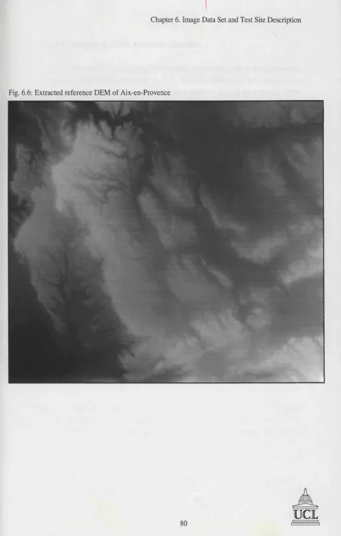
6.4 Reference DEM Introduction ... 78

Contents

7. Assessment of Stereo Matching Results

82

7.1 In tro d u ctio n ... 82

7.2 GRUEN and GRUENS Programme Analysis ... 83

7.3 Determination of Matching Strategy ... 86

7.4 Random Seed Points Generation ... 98

7.5 Random Seed Points Analysis ... 98

7.6 PDL File Data Testing ... 103

7.6.1 PDL file data testing: ORSE ... 103

7.6.2 PDL file data testing: GRSE ... 104

7.6.3 PDL file data testing: DEM accuracy for separated tie r 107 7.6.4 PDL file data testing: DEM accuracy and Image tie rs ... 108

7.6.5 PDL file data testing: comparison of two PDL f ile s ... 108

7.7 B lunder-rem oving ... 112

7.7.1 Global disparity analysis ... 113

7.7.2 Determination of threshold of blunder-removing filte r 114 7.7.3 Blunder-removing filter data testing ... 115

7.8 Techniques of Seed Points Selection ... 121

7.8.1 SEED_GRUEN programme introduction ... 121

7.8.2 Testing of two algorithms ... 123

7.8.3 Seed points selection by disparity sum ... 126

7.8.4 DEM accuracy of the disparity sum ... 126

7.9 Advantages of Pyramidal Stereo Matching Analysis ... 131

7.10 Performances of Matching on the Opposite-side Im agery... 134

7.11 Pyramidal Matching on the Speckle Reduction Im ag ery ... 138

7.12 Running Time Consideration ... 142

7.13 Sum m ary ... 143

8. Object Domain Approach

145

8.2 Geometric Constraint Conditions ... 146

8.3 Height Deviation and Constraint Condition ... 149

8.4 Determination of Constraint Condition ... 151

8.5 Characteristics of Constraint Values ... 162

8.6 Determination of Optimum Constraint Values ... 167

8.7 Analysis of DEM Accuracy by Geometric Constraint Conditions 170

8.8 Intersection Error Modelling by Image Coordinates ... 174

8.9.1 Using the coarse reference DEM ... 176

8.9.2 Using new derived DEM ... 182

8.10 Analysis of Success of Object Domain A pp ro ach... 184

8.11 Intersection Using the Control Points ... 185

8.11.1 Control points consideration ... 185

8.11.2 Range time calculation ... 186

8.11.3 DEM accuracy analysis ... 188

8.12 Sum m ary ... 192

9. Conclusion

194

9.2 Intersection A lgorithm ... 197

9.3 Overview of Achievements ... 199

9.4 F uture Studies ... 201

References

203

Appendix A: Least Squares Correlation Algorithm

210

Appendix B: Original Header Data File

213

Appendix C: Control Header Data File

217

List of Tables

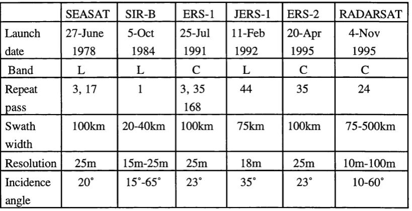
Table 2.1: Summary of principal characteristics of SAR sen so rs... Table 2.2: The period and repeat cycle duration for ERS-1 six main phase

Table 6.1 Table 6.2 Table 6.3 Table 7.1: Table 7.2: Table 7.3: Table 7.4: Table 7.5: Table 7.6 Table 7.7 Table 7.8 Table 7.9 Table 7.10: Table 7.11: Table 7.12: Table 7.13: Table 7.14: Table 7.15: Table 7.16: Table 7.17:

4 key data for the three images respectively •••• Definitions of three stereo pairs ... Offset of sample and line pixel for the test area

DEM accuracies (m) for the manual seed points under 3 different patch radius ... Coverage (%) for the manual seed points under 3 different patch radius ... RMS (m) for ERSP and DEM accuracy (m) for ORSE of PDLl and PDL2 under three different grid numbers ... RMS (m) for the growing random seed points of each t i e r ... DEM (m) accuracy for growing random seed points with two PDL files ... Coverage (%) for two PDL files without the R S E ... DEM accuracy (m) for the total and each t i e r ... Influence of image tier on DEM accuracy (m) and coverage (%) — The relationship of DEM accuracy (m) grand disparity sum (pixel) and height deviation (m) ... HDSE for two PDL files on tier4~8 under grid 3 2 ... HDSE, mean and RMS (m) for two PDL files under three

different grids ... The range and average of X and Y disparity (pixels) for three groups ... Range and average value of disparity sum (pixels) ... The upper and lower boundary of threshold value (pixel) of

disparity sum for different percentages ... The comparison of the final DEM accuracy (m) between five different types of threshold value and the original o n e ... The comparison of the HDSE between five different types of threshold value and the original one ... Coverage(%) of five different types of threshold value and the original one ...

Table 7.18: DEM accuracy (m) for five two-end boundaries, fixed at the lower boundary ... 118 Table 7.19: DEM accuracy (m) for three two-end boundary fixed at the upper

boundary ... 118 Table 7.20: The lower 100% threshold value (pixels)for two data s e ts 119 Table 7.21 : Number of (-) and (+)height deviation under three grid num ber 126 Table 7.22: Disparity sum (pixels) for ordinary and disparity seed points on

tier4 under three different grids ... 127 Table 7.23: Number of (-) and (+)height deviation under three grid number •— 127 Table 7.24 DEM accuracy (m) for ordinary and disparity seed points under

three different grids ... 127 Table 7.25: Comparisons of HDSE for ordinary and disparity seed points

under three different grid ... 128 Table 7.26: 100% lower boundary threshold value (pixels) for three sets of

disparity seed points under three different grids ... 128 Table 7.27: DEM accuracy (m) for the disparity seed points before and after

using blunder-rem oving filter ... 129 Table 7.28: Threshold values (pixel) computed by four different minus height

d ev iation ... 130 Table 7.29: Coverage(%) and DEM accuracy (m) by the four threshold values • 131 Table 7.30: DEM accuracy (m) comparison of different tiers for the original

and pyram idal image ... 132 Table 7.31 : DEM accuracy (m) of different seed_generation for the original

im age ... 132 Table 7.32: Proportion of grand_generation seed points for the original image

on each tier ... 133 Table 7.33: Coordinates of the growing seed points for image pyramid on

each tier ... 134 Table 7.34: DEM accuracy (m) and coverage(%) of five data sets of O P l 135 Table 7.35: DEM accuracy (m) and coverage(%) of five data sets of O P 2 136 Table 7.36: Coverage (%) for the larger eigenvalue for three sets of opposite

p air ... 136 Table 7.37: DEM accuracy (m) and coverage (%) for four sets of OPl d a ta 137 Table 7.38: DEM accuracy (m) and coverage (%) for four sets of OP2 d a ta 137 Table 7.39: DEM accuracy and coverage(%) for the original and

List of Tables

Table 8.1: 9 data sets selected for testing the relationship of constraint values

and height deviation ... 151

Table 8.2: 9 height deviation intervals and their corresponding statistics of

range error (m) of the same side stereo p a i r ... 151 Table 8.3: 9 height deviation intervals and their corresponding statistics of

range error (m) of the O Pl ... 152 Table 8.4: 9 height deviation intervals and their corresponding statistics of

range error(m) of the 0 P 2 ... 152 Table 8.5: 9 height deviation intervals and their corresponding statistics of

intersection angle (°) of the SA ... 153 Table 8.6: 9 height deviation intervals and their corresponding statistics of

intersection angle (°) of the O Pl ... 153 Table 8.7: 9 height deviation intervals and their corresponding statistics of

intersection angle (°) of OP2 ... 154 Table 8.8: Mean height deviation and the difference for two intervals of

extreme constraint values for SA ... 161 Table 8.9: Mean height deviation and the difference for two intervals of

extreme constraint values for O Pl ... 161 Table 8.10: Mean height deviation and the difference for two intervals of

extreme constraint values for 0P 2 ... 162 Table 8.11: Range error (m) of small height deviation for the same s id e 168 Table 8.12: Intersection angle (°) of small height deviation for the O P l 168 Table 8.13: Intersection angle (°) of small height deviation for the O P 2 168 Table 8.14: DEM accuracy (m) comparison for the optimum ranges or

optimum values of range error for the SA ... 169 Table 8.15: DEM accuracy (m) comparison for the optimum ranges or

optimum values of intersection angle (°) for the O Pl ... 169 Table 8.16: DEM accuracy (m) comparison for the optimum ranges or

optimum values of intersection angle for the O P 2 ... 169 Table 8.17: DEM accuracy (m) and HDSE comparison between the original

and constraint condition for SA ... 171 Table 8.18: DEM accuracy (m) and HDSE comparison between the original

and constraint condition for O Pl ... 171 Table 8.19: DEM accuracy (m) and HDSE comparison between the original

and constraint condition for OP2 ... 172 Table 8.20: Gradient of errors in intersection with respect to 3 coordinates

Table 8.21: Gradient of errors in intersection with respect to 3 coordinates

by shifting one pixel in Y direction ... 174 Table 8.22: Gradient of total errors in intersection of shifting one pixel in

X and Y direction... 175 Table 8.23: Convergence angle (°) and intersection angle (°) for three stereo

pairs ... 175 Table 8.24: The DEM accuracy (m) and HDSE of five data sets by the standard

height approach (coarse reference DEM) for S A ... 177 Table 8.25: DEM accuracy (m) and HDSE of five data sets by the standard

height approach (coarse reference DEM) for OPl ... 181 Table 8.26: DEM accuracy (m) and HDSE of five data sets by the standard

height approach (coarse reference DEM) for OP2 ... 181 Table 8.27: The DEM accuracy (m) and HDSE of five data sets by the standard

height approach (new reference DEM) for SA ... 182 Table 8.28: The DEM accuracy (m) and HDSE of five data sets by the standard

height approach (new reference DEM) for O Pl ... 182 Table 8.29: The DEM accuracy (m) and HDSE of five data sets by the standard

height approach (new reference DEM) for OP2 ... 184 Table 8.30: Lambert Zone 3 coordinates of 3 control points ... 188 Table 8.31 : The DEM accuracy (m) and HDSE of five data sets by using

3 control points for SA ... 188 Table 8.32: The DEM accuracy (m) and HDSE of five data sets by using

3 control points for O Pl ... 189 Table 8.33: The DEM accuracy (m) and HDSE of five data sets by using

3 control points for 0 P 2 ... 189 Table 8.34: The ground coordinates of the intersection of control points using

the original and control header data file for SA... 190 Table 8.35: The ground coordinates of the intersection of control points using

the original and control header data file for O Pl ... 190 Table 8.36: The ground coordinates of the intersection of control points using

the original and control header data file for O P 2 ... 190 Table 8.37: Statistics of height difference(m) between the DEM with and

without control points for SA ... 191 Table 8.38: Statistics of height difference (m) between the DEM with and

without control points for O Pl ... 192 Table 8.39: Statistics of height difference (m) between the DEM with and

without control points for OP2 ... 192

List of Figures

Figure 2.1: Locations and coverage zone of ERS-1 ground receiving stations-•• 26 Figure 2.2: Dependence of the azimuth resolution (Ra) on antenna

beamwidth(P) and ground range ... 31

Figure 2.3: Doppler history of a point target ... 32

Figure 2.4: Geometry of a synthetic aperture array ... 33

Figure 2.5: Flow chart of SAR image processing using the frequency domain approach ... 35

Figure 3.1: Geometric distortions due to the terrain elevation effects 39 Figure 3.2: Definitions in object space for the vertical exaggeration of camera stereo m odel ... 41

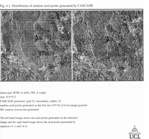
Figure 4.1: Random seed points distribution on SA ... 55

Figure 4.2: An example of PDL file ... 56

Figure 4.3: CHEOPS pyramidal matching flow chart ... 58

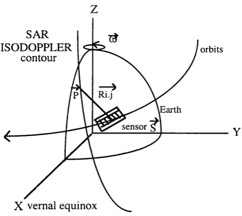
Figure 5.1: Geocentric inertial system ... 66

Figure 5.2: Intersection flow chart ... 67

Figure 5.3: Relationship between inertial system and geocentric terrestrial system ... 70

Figure 6.1: RTM_A raw image ... 75

Figure 6.2: PRI_A raw image ... 76

Figure 6.3: PRI_D raw image ... 77

Figure 6.4: Location of test area in France ... 74

Figure 6.5: Extracted reference DEM boundary ... 79

Figure 6.6: Extracted reference DEM of Aix-en-Provence ... 80

Figure 7.1 : Three numerical examples of 12 values of GRUEN’s ou tp u t 85 Figure 7.2: P D L l file ... 88

Figure 7.3: PDL2 file ... 89

Figure 7.4: Strategy 1 execution procedures ... 90

Figure 7.5: Numerical example for strategy 1 ... 91

Figure 7.6: Strategy 2 execution procedures ... 92

Figure 7.7: Numerical example for strategy 2 ... 93

Figure 7.9; Perspective view of DEM from manual seed points matching

(radius 20) ... 96

Figure 7.10: Perspective view of DEM from manual seed points matching (radius 25) ... 97

Figure 7.11: Flow chart of GRUENS_SEED ... 101

Figure 7.12: Diagram for the techniques of the GRUENS_SEED... 102

Figure 7.13: The comparison of DEM accuracy between the original and lower threshold for three data sets ... 120

Figure 7.14: The comparison of DEM accuracy between the original and lower threshold without the ERSP for three data sets ... 120

Figure 7.15: Flow chart of SEED_GRUEN programme ... 124

Figure 7.16: Flow charts for two matching scripts ... 125

Figure 7.17: Comparisons of DEM accuracy improvements under three grid num ber ... 129

Figure 7.18: LEE filtered image matching coverage ... 139

Figure 7.19: MAP filtered image matching coverage ... 140

Figure 7.20: Original image matching coverage ... 141

Figure 8.1: Geometric constraint condition the same side stereo p a ir 147 Figure 8.2: Geometric constraint condition the opposite side stereo p a ir 147 Figure 8.3: Relationship of range error (m) and height deviation for the SA ••• 154 Figure 8.4: Relationship of range error (m) and height deviation for the OPl •• 155 Figure 8.5: Relationship of range error (m) and height deviation for the OP2 •• 155 Figure 8.6: Relationship of intersection angle (°) and height deviation for the SA ... 156

Figure 8.7: Relationship of intersection angle (°) and height deviation for the O P l ... 156

Figure 8.8: Relationship of intersection angle(°) and height deviation for the OP2 ... 157

Figure 8.9: Extent of range error (m) under different height deviation (m) for the SA ... 158

Figure 8.10: Extent of intersection angle(°) under different height deviation (m) for the SA ... 158

Figure 8.11: Extent of range error (m) under different height deviation (m) for the O P l ... 159

Figure 8.12: Extent of intersection angle (°) under different height deviation (m) for the O P l ... 159

List of Figures

Figure 8.14: Extent of intersection angle (°) under different height deviation (m)

Figure 8.15 Figure 8.16 Figure 8.17 Figure 8.18

for the 0 P 2 ... 160 Range error (m) of SA with respect to the X coordinate... 164 Range error (m) of SA with respect to the Y coordinate... 164 Range error (m) of SA with respect to the X+Y coordinate 165 Intersection angle (°) for the opposite side with respect to X

coordinate ... 165

Figure 8.19: Intersection angle (°) for the opposite side with respect to Y

co o rdinate ... 166 Figure 8.20: Intersection angle (°) for the opposite side with respect to

X+Y coordinate ... 166 Figure 8.21: Perspective view of original DEM of same s id e ... 178 Figure 8.22: Perspective view of geometric constraint DEM of same s id e 179 Figure 8.23: Perspective view of extracted reference Aix-en-Provence DEM 180 Figure 8.24: Perspective view of standard height approach DEM

First of all, I would like to express my sincere thanks to Prof. I.J. Dowman for his supervision and instruction over these past four years. I also thank Prof. J.P. Muller for his guidance and help during this study. I also feel grateful to Mark Upton for his kind assistance in teaching me to use some helpful computer commands. My thanks also go to Chrystelle Ourzik and Jeremy Morley for they show me how to draw beautiful figures for this thesis.

English academic writing is a difficult work for me and here I appreciate Isabella's help to correct my poor English writing and Paul Dare to proof-read my thesis. I also show my gratitude to Ms. Wu and Mr. Tickell who have allowed me to use their PC for without them, this thesis would not have been completed so quickly.

I honestly thank my family in Taiwan for their encouragement and endurance of my absence during these past four years. Without their moral support, this thesis would not be finished. Special thanks must go to my wife for her looking after the whole family alone in Taiwan for such a long time.

Abbreviations

ALSC; Adaptive Least Squares Correlation AMI; Active Microwave Instrument

CSA: Canadian Space Agency

EECF: Earthnet ERS-1 Central Facilities ERS-1: European Remote Sensing satellite ERSP: Effective Random Seed Points ESA: European Space Agency

EFT: Fast Fourier Transform

GRSE: Growing Random Seed Effects GMST: Greenwich Mean Sidereal Time GAST: Greenwich Apparent Sidereal Time GCP: Ground Control Points

HER: High Bit Rate

HDSE: Height Deviation Shifting Effect ID: Julian Date

JPL: Jet Propulsion Laboratory LBR: Low Bit Rate

LFM: Linear Frequency Modulated LSC: Least Squares Correlation

MSEC: Mean Square Error on the Contrast MHD: Mean Height Difference

MMCC: Mission Management and Control Center NCC: Normalised Correlation Coefficient

DIE: Original Image Effect

OPl: Opposite stereo Pair - PRI_D (left), PRI_A (right) OP2: Opposite stereo Pair - PRI_D (left), RTM_A (right) ORSE: Original Random Seed Effect

PAF: Processing and Archiving Facilities PDL: Pyramidal Description Language PRJ: Precision SAR Imagery

PRI_A: PRI Ascending ERS-1 image PRJ_D: PRI Descending ERS-1 image PRF: Pulse Repetition Frequency RSE: Random Seed Effects

RTM_A: RTM Ascending ERS-1 Image

SA; Same side stereo pair - RTM_A (left), PRI_A (right) SIHE: Systematic Increasing Height Effects

Abstract

This research was concerned with various aspects of deriving DEM information from ERS-1 SAR imagery. Stereoscopic SAR offers the possibility to determine a DEM of large areas and is complementary to interferometric SAR (IFSAR). Compared with former SAR image data sources, ERS-1 has the advantage of providing accurate ephemeris data. In addition, it has different image modes which enables the verification of results from various research groups regarding geometric configurations. One of the aims of this study was to establish a standard model for deriving DEM accuracy, based on ERS-1 as the image data source, that would be applicable for all other new types of SAR imageries. An example of such SAR imageries worth investigating in the future is RADARSAT, which provides versatile image modes with a wide range of incident angle and resolution.

In summary, the studies carried out for this research project could be described under two subheadings, namely matching and intersection. With respect to the matching, pyramidal stereo matching techniques were used in combination with an excellent area-based region growing algorithm to achieve dense coverage. The special interest in this study is the initial seed points used for the pyramidal matching process employed were chosen randomly instead of by manual selection. To examine the function of these random seed points, the original matching algorithm was modified to have four extra values in its output, which were later found to be able to aid the determination of the advantages of using image pyramids. It was also discovered that the disparity sum was a good measure forjudging the factors affecting the matching accuracy in most of the studies. As a result, this parameter was used to investigate different strategies of pyramidal matching, to pin-point the link between the upper and lower tier in the image pyramid, as well as for the removal of the blunders.

It is demonstrated in this thesis that with a same side convergence angle of 2.14°, the intersection error could reach 426.95m for one Y pixel shift. The above phenomenon explains the underlying reason why the DEM accuracy could not be improved to the same accuracy as, for example, SPOT data.

To summarise, a satisfactory DEM could be obtained from ERS-1 images using the approaches developed in this study which could reach an accuracy of 20.18m for the same side and 12.23m for the opposite side with the coverage of better than 80%. However, the orbit information unique to ERS-1 was observed to play an important role in the accuracy of DEM derived using the methods developed. If this information was not provided, other rigorous alternatives are required for its determination and these were investigated.

CHAPTER 1

Introduction

1.1 Introduction

The use of the radar imagery can be dated back to the World War II for reconnaissance. It was later adopted for topographic mapping in the early 1970s, when the US Engineers of Army Corps initiated a series of studies that became the basis for current radargrammetry. 1:25000 maps could be generated for entire countries, for example, maps were obtained for Brazil and Venezuela in 1971 and

1979 respectively.

The development of imaging SAR has progressed rapidly, since the techniques of converting signals received from the SAR could be improved digitally. From 1978 onwards, SAR imagery data has mainly been derived from space satellites such as SEASAT, SIR-A, and SIR-B. SEASAT focused mainly on the global ocean surface. Despite the fact that it only remained operational for several months, numerous images of the Earth surface were recorded to demonstrate the possibility of using satellite imageries to monitor the Earth surface. The SIR-B is another important mission leading to many important studies, including rectification [Goodenenough et al., 1979], image stereo matching [Ramapryan et al., 1986], as well as the analysis of optimum look angles for stereo viewing [Thomas at al., 1987]. The tendency of using satellite radar imagery for various applications has become apparent in recent years, as more satellites carrying SAR have been launched, including NASA's Venus radar mapping mission Magellan, ERS-1, SIR-C, RADARSAT, and JERS-1. ERS-1 is the image data source utilised in this study and this satellite, along with RADARSAT, will be introduced in the next chapter.

1.2 Overview

The authors made the conclusion that SAR had a potential for small scale mapping and map revision, but more work was required to validate this proposal. From then on, a spectrum of studies related to radar image mapping were carried out, from the introduction of intersection [Leberl, 1976], the derivation of error modelling [Leberl, 1979], to the investigation of algorithms used for the automatic matching [Leberl, 1994]. In UCL, a series of studies on radar image mapping has been carried out over the years, and one of the remarkable achievements was the proposition of the analytic method as a mathematical model for intersection. This method was originally proposed in Clark's Ph.D. thesis to geocode SlR-B imagery and was subsequently used in an intersection algorithm for manual check points on different stereo pairs of ERS-1 images. Valuable conclusions were drawn based on Clark’s work, and one of the objectives of this study was to further evaluate her findings by testing with more matching results.

Lately, most of the studies regarding radar image mapping have incorporated another sophisticated technique named interferometry to derive a Digital Elevation Model (DEM). This technique was developed in the Jet Propulsion Laboratory (JPL) in 1974, and it uses two complex SAR image data acquired by the two passes separated by the multiple of a repeat cycle to calculate the phase difference between two corresponding image points. Based on existing knowledge regarding orbit parameters, the phase difference can be related directly to the altitude on a pixel by pixel basis to generate DEMs. Unlike stereoscopic SAR, this technique deals with pixel phase rather than its intensity. Interferometry is believed to give better DEMs, but the technique still has unresolved problems and has not been proved over a wide range of land cover and atmospheric conditions. This is evident in the latest study undertaken by Kenyi and Raggam [Kenyi and Raggam, 1996], in which the accuracy of the generated DEM could achieve a Root Mean Square Error (RMSE) of 9m by using control points.

The studies described above have illustrated that radar image mapping is a promising subject worth investigating. In addition, it offers the following advantages:

1) it is an active sensor and the illumination can be controlled at specified incidence angles, which may produce overlapping images suitable for mapping.

2) its resolution is independent of the distance to the object.

3) it can penetrate surface layers of snow [Leberl, 1990] and vegetation, which is important for some areas that can not be covered by other sensors, such as the polar region.

Chapter 1. Introduction

Despite the advantages described above, some drawbacks do exist in several aspects in the application of radar image mapping. Instead of processing digital image data directly by using normal computer workstations that are more feasible and can be easily modified to suit other image types, some studies actually employed more expensive and inflexible analytic stereo plotters [Leberl, 1988] and other digital stereo workstations [Toutin, 1996]. In addition, due to the lack of the orbit information, the geometric modelling for most studies was completed by selecting ground control points followed by the employment of less reliable polynomial functions. Moreover, almost all evaluation of the final derived DEM from SAR carried out in the past were based only on a small number (<100) of selected points instead of comparing on a large scale (e.g. DEMs).

1.3 Aims

The main purpose of this study was to develop an automatic approach to establish a standard model that is able to derive DEM information with great accuracy from the stereoscopic SAR imagery, and to subsequently investigate its potential and limitations. The methods developed in this study were validated using the ERS-1 image data, but they should also be applicable to other similar new radar images e.g. RADARSAT.

Considering both the advantages and the problems yet to be solved regarding the use of radargrammetry, this study aimed to achieve the following objectives :

(1) Assessment of an existing automatic matching algorithm, combined with a) the use of random seed points and b) the sophisticated area-based GRUENS algorithm, to determine its ability to create DEMs with dense coverage as well as greater accuracy from radar imagery automatically.

(2) Evaluation of the analytic intersection algorithm by using the Doppler equation and range equation to obtain the terrain height. This new approach utilises the header data available without the requirement of control points. In addition, a comparison of the new approach with other imagery previously completed by other research groups would be carried out.

(4) Evaluation of the feasibility of deriving DEMs from the SAR imagery. This was achieved by comparing numerous matching points on a large scale, instead of a small number of selected points as generally done in the past.

(5) Investigation and validation of the geometric conditions for stereo pairs under different situations and for which purpose, three stereo pairs, namely the same side and the two opposite sides, were included in this study.

(6) Utilising a normal computer workstation facility to prove the feasibility of deriving a DEM from SAR imagery without any analytic stereoscopic workstations, which could provide a good example for generating reliable results at affordable cost.

1.4 Outline of This Thesis

Chapter 1. Introduction

CHAPTER 2

SAR Sensors and Data Products

2.1 Introduction

In this chapter, background information on ERS-1 and other conunon sensors is introduced to provide a context for this study. The principal characteristics of these sensors are listed in Table 2.1. The image formation of SAR imagery is rather complicated compared to the traditional optical imagery. To facilitate a better understanding of SAR imagery, an overview of its image formation process is provided in this chapter. Backscattering of the radar signal is also analysed here along with some fundamental concepts on the principles of SAR images. In the last section, there is a brief outline on geocoding techniques.

SEASAT SIR-B ERS-1 JERS-1 ERS-2 RADARSAT

Launch date

27-June 1978

5-Oct 1984

25-Jul 1991

11-Feb 1992

20-Apr 1995

4-Nov 1995

Band L L C L C C

Repeat pass

3, 17 1 3, 35

168

44 35 24

Swath width

100km 20-40km 100km 75km 100km 75-500km

Resolution 25m 15m-25m 25m 18m 25m 10m-100m

Incidence angle

20° 15°-65° 23° 35° 23° 10-60°

Table 2.1: Summary of principal characteristics of SAR sensors

2.2. ERS-1: Overview

2.2.1 Introduction

Chapter 2. SAR Sensors and Data Products

the antenna folded its size is approximately 12m*12m*2.5m, weighting 2400kg, which makes it the largest and most sophisticated free-flying satellite ever built in Europe. ERS-1 is a forerunner of a new generation of satellites for environmental monitoring.

Compared with other contemporary satellite systems, ERS-1 has many advantages. It has the ability to meet several operational requirements for data products requested within a few hours of observations. This ability enables ERS-1 to make significant contributions to meteorology, sea state forecasting and monitoring of sea ice distribution. In addition, the stability of the ERS-1 orbit has shown a new direction in using the interferometric technique for cartography application. Another advantage of ERS-1 is that it could gather data from remote areas such as the polar regions and the southern oceans where little information has been collected before.

2.2.2 ERS-1 missions

The ERS-1 specific mission objectives are both scientific and operational. It aims to provide users with Earth observation data for a wide variety of applications and this can be achieved by its pre-determined global coverage. The main targets of the ERS-1 mission are oceans and sea-ice zones at global scale as well as some coastal areas of interest.

In order to meet the various objectives of its missions, the ERS-1 was planned to move around the Earth in a elliptical sun-synchronous polar orbit. For different purposes, ERS-1 has 8 main phases. The fundamental data of these 8 phases are listed in Table 2.2:

Mission Phase Period Repeat

orbit acquisition 17.07.91-30.07.91 3-day commissioning 26.07.91-10.12.91 3-day first ice 28.12.91-30.03.92 3-day roU-tilt mode 02.04.92-14.04.92 35-day multi-disciplinary 14.04.92-15.12.93 35-day second ice 01.01.94-31.03.94 3-day

geodetic 28.09.94-21.03.95 168-day

tandem 21.03.95-06.05.96 35-day

In the above 8 phases, the last long phase was introduced primarily to support the oceanographic applications without orbit disturbance. Another important campaign that was Roll-Tilt mode imaging. In this mode, the Earth was imaged by a larger incidence angle (35° instead of 23°) for a short period (4-13 April, 1992). This Roll- Tilt mode image is crucial for stereoscopic SAR, because it provides a good opportunity to evaluate the impacts of intersection angles on the results of intersection by its larger incidence angle. Results of testing them will be shown in Chapter 8.

On the ERS-1, the payload consists of active and passive microwave sensors and a thermal infrared radiometer, of which the Active Microwave Instrument (AMI) is the most important for mapping. AMI combines the functions of SAR and a Wind Scatterometer. The SAR operates in image mode for acquisition of wide-swath, all weather images over oceans, polar regions, coastal zones and land under all-weather conditions. This is named high bit rate mission (HER). In the HER, as the data rate is too high for on-board storage, it is only acquired within the reception zone of suitably equipped ground receiving stations. In contrast to the high bit rate mission, the low bit rate mission (LER) was operated globally which consists of Radar Altimeter, Along Track Scaning Radiometer, AMI Wind Scatterometer, and AMI SAR in Wave Mode. Since LER is of a global nature, along each orbit, the LER data are stored on board then dumped to one of the ground receiving stations before the next orbit. The high bit rate mission is in particular demand since it is driven by the request of users and is constrained by the actual operations of the ground stations around the world. Therefore, this mission requires careful planning in advance.

In this study, we only used the SAR imagery as our data source, therefore, the above mentioned SAR image acquisition should be introduced further here. SAR data can only be acquired for a maximum duration of approximately 12 minutes per orbit. The rectangular antenna of the SAR directs the narrow beam sideways and downward onto the Earth surface to obtain strips of high resolution imagery of about 100km in width. This high resolution imagery is obtained through a series of image processing techniques which will be introduced in later sections.

2.2.3 ERS-1 ground segment

Chapter 2. SAR Sensors and Data Products

is located in Darmstadt, Germany and named the Mission Management and Control Center (MMCC). MMCC monitors and controls the spacecraft and schedules its payload operation through the ground station in Kiruna. The Earthnet ERS-1 Central Facility (EECF) is located in Italy, which carries out all user interface functions and is also responsible for data coordination, dissemination as well as quality control. In ground stations around the world acquire the ERS-1 data almost routinely, meanwhile they also process and disseminate the fast-delivery products. The locations of these ground receiving stations (1993, September) as well as their coverage zones to are shown in Fig. 2.1. There are four Processing and Archiving Facilities (PAE), located in Germany, France, Italy and Great Britain respectively. The PAF deal mainly with off-line precision products and the archiving and distribution of ERS-1 data.

2.3 ERS-1 Data Products

2.1: L ocations and coverage zone o f ERS-1 ground receiving stations

cu

^ q . H O /

Key:

ESA Stations

KS Kiruna. Sw eden FS

MS M aspaio mas, Spain GS

PS Prince Albert L ow Rate. C a n a d a

National Stations

G H Gatinea u High Rate. C a n a d a PH

T O Aussaguel. Fra nce T F

TS Tro m so. N o rw a y W F

LI Libreville. G abon

(G erm an T ra n s p o r ta b le Station)

Foreign Stations

A F Fairbanks. U SA AS

A T Atlanta Test Site. U S A BE

C O Cotopaxi. E q u a d o r C U

HA Hatoyama. Japan H O

IN Pare-pare. In d o n es ia IS

KU K umamoto. Japan SA

SE Hyderabad. India SY

T H Bangkok. Th ailan d

Fucino. Ital>'

G a tin e a u L o w Rate. C a n a d a

Prince A lb e rt High Rate. C a n a d a O ’H ig g in s i A n tarctica). G e rm a n y W e s t F r e u s h . UK

Alice S p rin g s. .Australia Beijing. C h in a

Chapter 2. SAR Sensors and Data Products

2.4 RADARSAT Overview

RADARS AT is a sophisticated Earth observation satellite developed by Canada to support the operational needs mainly on environmental monitoring and other related fields such as agriculture, cartography and hydrology The satellite was launched on November 4 in 1995 on a Delta II rocket and is expected to last for 5 years. RADARSAT will provide Canada as well as the world with a large amount of timely- delivered data which will meet the needs of environmental and resource professionals worldwide.

RADARSAT was developed under the management of the Canadian Space Agency (CSA) with strong support from industry (e.g. Spar Aerospace, CAL Corporation), provincial governments (e.g. Quebec, Ontario), international partnership (e.g. NASA) for the launch platform as well as other approximate 100 or so organisations in Canada. The CSA is responsible for the design and integration of the overall system for its control and operation. The data reception and processing are carried out in the ground receiving stations located in three different provinces and states in Canada and United States including. Prince Albert, Saskatchewan; Gatineau, Quebec; and Fairbanks, Alsaka. .

RADARSAT carries only one SAR instrument and operates in C-band like the ERS-1. While in operation it will provide more choices in the manner for which the images are acquired. The image swath can vary from 35km to 500km giving rise to corresponding image resolution ranging from 10m to 100m. Incidence angles can be altered from less then 20° to more than 50°. RADARSAT provides global coverage with the flexibility to fulfil specific requirements. It can cover the Arctic daily regardless of the weather condition and most of Canada every 24 hours depending on the swath selected. The entire Earth would be covered every 24 days using the standard 100km wide swath. The coverage of the Arctic area is of special importance for some shipping companies and government agencies who need to deal with ice reconnaissance.

RADARSAT can capture up to 28min worth of data covering up to 1.1 million square kilometres of the Earth's surface. For convenience of users, the data can either be down-linked in real time or stored on one of the two tape recorders until the spacecraft is within the range of a receiving station. To satisfy users who require timely data, the RADARSAT processing system can deliver data to on-line users within a few hours after the satellite has passed over an area. There are three main types of imaging data acquired by RADARSAT including the quick look, georeference, and geocoded data. Quick look consists of uncorrected images, while georeferenced products are geometrically corrected to compensate for the Earth curvature. The geocoded products on the other hand are rectified on a standard map projection.

2.5 SEASAT, SIR-A, SIR-B and SIR-C Overview

In 1978, SEASAT was launched by NASA to develop global coverage with a radar imaging sensor that operated at L-band (25cm wavelength). Unfortunately, it was only operational for three months due to fatal defects on board of the satellite. Within the three months though, many coverages were obtained over land and Arctic regions and were very useful for research work on radar image mapping. This encouraged NASA to carry out another spacebome radar imagery experiment. SIR-A (Shuttle Imaging Radar) carried by the space shuttle Columbia. It was launched in 1981 and it was also operated at L-band with primary use in exploring geological mapping. SIR-A obtained images at the selected incidence angle of 50° so that the acquired backscattering are dominated mainly by the surface roughness, which was helpful for the interpretation.

Chapter 2. SAR Sensors and Data Products

photogrammetric plotter. The resulting height accuracy was ±98m, which is about ±2.5 times of the image resolution element.

A further NASA space shuttle mission was launched in 1984 labelled SIR-B. It had many similarities to SIR-A in its system design, however, with a major difference in the image recording system. Unlike SIR-A, it could convert the signals received to images using a digital correlator. In addition, the slant range resolution of SIR-B was better than SIR-A, being 15m and 40m respectively. Another important feature of SIR-B is that it could vary the look angle. This is important with respect to radar image mapping, for it could provide image stereo pairs with different intersection angles so that different geometric conditions could be examined. This feature subsequently demonstrated how incidence angle could influence the capability of interpretation of various terrain features.

The Shuttle Imaging Radar-C (SIR-C) was the third in a series of space shuttle based Synthetic Aperture Radars sponsored by NASA designed to fly on a low Earth orbit. Unlike the SIR-A and SIR-B that operated at the single L-band and had single horizontal polarisation, SIR-C was a dual-frequency quad-polarisation radar operating at both L band and C band frequencies. The SIR-C was important for being the first instrument that could provide the multiseason coverage of a multiparameter imaging radar. The image data was collected over incidence angles from 17° to 63°.

2.6 SAR Fundamental Principles

An imaging radar works by transmiting its energy to scan the earth’s surface. The transmission of energy is by means of radio microwave at the rate of pulse repetition frequency (FRF), emitted by the sensor. The bandwidths of the imaging radar determines the magnitude of range resolution. In imaging radar, two resolutions are considered with respect to two different directions. The range resolution is on the direction of the energy propagation, which is also called the range direction or across- track. The other direction is related to the flight direction of the sensor named azimuth or along-track direction.

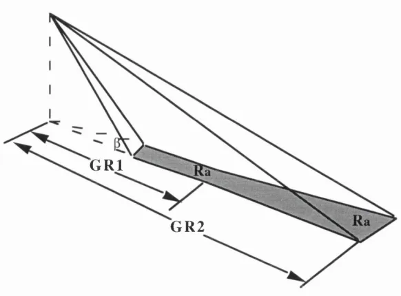
Considering the azimuth resolution at a given range as shown in Fig. 2.2, it is determined by the angular beam width

P

Ra=R.P

(2-1)

where:

Rai the azimuth resolution P : beam width of the antenna R: range distance

The beam width of antenna

P

P=X/L

(2-2)

where:

X : wave length

L : physical length of the antenna

combining (2-1) and (2-1), becomes

R^=R*X/L (2-3)

Chapter 2. SAR Sensors and Data Products

G R l

GR2

Fig. 2.2: D ependence of the azim uth resolution (Ra) on antenna beam w idth(P ) and ground range (GR)

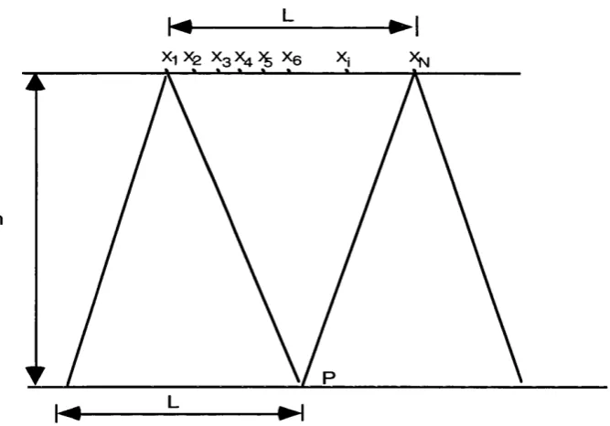
In SA R, for each object point P, the antenna transm its a pulse and records the returned echo along the flight track at each position. The D oppler shift o f the echo from P will be firstly positive, then decreases to zero, then becom es increasingly negative until P exits from the beam (see Fig. 2.3). The zero D oppler will give the tim e at w hich the target is perpendicular to the azim uth. By recording the D oppler shift history and com paring with reference frequency allows m any returned echoes to be focused on one single point. This function is equally used to sim ulate the effective length o f the antenna as the distance travelled by the signals sent out from the antenna (see Fig. 2.4). As a result, the azim uth resolution is independent o f the range betw een the sensor and the object and is only proportional to the size o f the physical antenna.

2.7 R adar Backscattering

Sensor track

P

Fig. 2.3: Doppler history of a point target (after [Elachi, 1988])

well as the wavelength can all be controlled by the radar designer, all except one variable, the radar cross-section ( a ). Therefore it is the factor which is of great importance in distinguishing the targets. Targets which may in all other respects be completely different can not be distinguished if they have the same backscatter.

S = PtOVg

(47u)3r4 _(2-4)

where:

S : returning signal Pt: transmitted power G : antenna gain ^ : wavelength

a : radar cross section

R : distance from the antenna to the target

Chapter 2. SAR Sensors and Data Products

X-| X3 Xg

h

L

Fig. 2.4: Geometry of a synthetic aperture array. Point P is visible from locations X i to Xn. The length of the synthetic aperture is equal to the real antenna footprint L. (After [Elachi, 1988])

2.8 SAR Image Processing

For the imaging radar, the transformation of the obtained object signal to images is rather an important aspect to be considered in this study. Overall, these transformations can be proceeded in two directions, either optical or digital, and both methods involve a series of complex procedures. In this study, only digital image processing was considered and its general concept should be introduced. Notice here that, the real situation of interaction between the sensor movement and the object has not been dealt with in this study. Rather, the start-stop approximation was adopted, which assumed that the radar platform remained stationary while transmitting and receiving the pulse. After the sensor moves to a new position, it will again remain stationary while transmitting or receiving the next pulse.

SAR digital image processing is mainly performed in the frequency domain to reduce the number of arithmetic operations. It consists of a sequence of convolution operations and a flow chart of the whole digital image process is shown in Fig. 2.5. Each step will be further introduced in the following subsections.

Chapter 2. SAR Sensors and Data Products

FFT

FFT

in v erse FFT c o rn e r tu rn in v e rse FFT

a z i m u t h r e f e r e n c e

r a n g e r e f e r e n c e

a z im u th c o m p re s s io n ra n g e c o m p re ssio n

ra n g e m ig ra tio n c o rre c tio n

o u t p u t

Fig. 2.5: Flow chart of SAR image processing using the frequency domain approach

2.9 SAR Geocoding

For SAR imagery, apart from layover, foreshortening, and shadow effects introduced earlier, is still affected by a number of radiometric and geometric distortions caused by the terrain relief which could prevent the effective utilisation of imagery. The elimination of these distortions is very important in many applications of remote sensing, such as multitemporal change detection. The procedure that is able to remove the distortion specifically for SAR imagery is named geocoding.

requires a large number of control points (GCP) in the image to allow the computation of polynomial coefficients of the mapping function. The outcome of this geocoded image is heavily dependent on the quality of the GCP. A general review of this method can be found [Naraghi et al., 1983]. The advantages of this method is that it does not need the ephemeris data. Noted that this method is best used for flat regions, as it is unable to deal with areas with varying terrain relief.

Parametric method attempt to model the geometry relationship of the image and object space [Meier and Nuesch, 1985]. The relationship can be described by the Doppler equation and range equation. In other words, for each image point, a set of Doppler and range equation can be constituted for derivation of the target coordinates. Similar to resection in Photogrammetry employed to calculate the exterior orientation, here, we measure the coordinates of control points in object space in order to predict the sensor position, velocity etc.. The above two equations are nonlinear, so the unknowns are solved by an iteration technique. After each iteration, the consistency of the two equations are checked by the updated parameters of sensors and when the residuals of the two equations are below a pre-determined limit, the process is terminated. Then each image point can be transformed into the map reference system by using these calculated Doppler and range equations. This method still has a disadvantage, in that it requires a large number of very good GCPs and the preliminary data of sensor must be rather accurate, otherwise, the problem of non­ convergence will occur.

If orbit information is available, the SAR range-Doppler methods can be used to proceed the geocoding [Noack et al., 1987]. This method also takes advantage of the above two equations, but unlike the previous method, it will further implement the variation of Doppler frequency in the geocoding. For it will fully employ auxiliary information (e.g. orbit parameters), so a minimal number of GCPs will be required. Since for ERS-1, orbit information will be provided in the header file, this method is said to be suitable to geocode ERS-1 image data [Clark, 1991].

Chapter 2. SAR Sensors and Data Products

for this standard ellipsoid geocoding, [Roth et ah, 1993], however, the outcome will still suffer from the terrain effects.

After the geocoding procedures has been completed, the rectified image pixels may be on non-integer positions for which the grey value needs to be recalculated by the bilinear resampling function. Notice that this resampling procedures will also degrade radiometric image quality, great care therefore must be taken when analysing the geocoded products.

2.10 Summary

Stereoscopy Using SAR Imagery

3.1 Introduction

This chapter gives a general introduction to several aspects of SAR imagery, including image characteristics and stereoscopy, that are related to stereo matching. A sound understanding of these subjects is the basis for further research in this study. Three preliminary SAR image characteristics will be mentioned in the first section, followed by an illustration of the concept of stereoscopy, focusing especially on SAR imagery. The exaggeration factor would also be analysed and the elements that influence the viewing ability are summarised. A general discussion on speckle- removing filters is included here. Finally, attention will be drawn to the difficulties in stereo matching that were encountered.

3.2 SAR Image Characteristics

For an imaging radar, due to the principles of acquiring the image, terrain relief will introduce geometric as well as radiometric distortions. These distortions observed in SAR imagery, then affect the matching, interpretation as well as other applications. Therefore, the characteristics of SAR are introduced here before proceeding to practical work shown in Chapter 7 and 8.

When a vertical feature is encountered by a radar pulse, if the top of the feature is reached before the base, then layover is said to occur and the top is closer to the nadir than the base on the imagery. This situation occurs whenever the terrain slope is steeper than the depression angle. The layover effect is most severe in the near image and gradually decreases towards the far range [Lillesand and Kiefer, 1994]. If on the contrary, when the terrain slope is less steep than the depression angle, then foreshortening effects instead of the layover will take place, which will cause the slope of the surface to become compressed on the image. Its severity increases as the steepness of the slope approaches perpendicularly to the depression direction.

Chapter 3. Stereoscopy Using SAR Imagery

shadow frequently occurs on hill slopes, that are facing away from the radar antenna and as a result receiving weak signal or no signal at all. The phenomenon could also be explained by the relationship of depression angle and the back slopes, such that the shadow effect occurs when the latter is steeper than the former. The shadow length will increase with range due to the decrease in the depression angle, which in turn means the shadow is proportional to the incidence angle. The radar shadow is an important factor in interpretation, particularly for geological application. In paper [Kaupp et al., 1982], the author simulated SAR imagery with different incidence angles and concluded that large incidence angles are better for geological applications, for it not only minimises the geometric distortions but also causes large shadows that could provide enhancement of topographic relief. The distortions of layover, foreshortening and shadow are shown in Fig. 3.1.

Slant Range _{1 2 4 3}A B ₅ C ₆

Sensor Altitude

A: Foreshortening B: Layover C: Shadowing

Earth Surface

2

1 3 4 5 6

B

Fig. 3.1: Geometric distortions due to the terrain elevation effects (after (Schreier, 1993])

3.3 SAR Stereoscopy

different geometric structure. For example, the parallax resulting from a topographic feature will be completely different from that of the airphotoes by the camera. To explore this difference, various aspects of the stereoscopic condition should be discussed first. Initial work on radar stereoscopy was carried out by LaPrade. In his paper [LaPrade, 1972], determined the optimum flight configurations for airborne radar by keeping the parallax constant for all images. LaPrade also was the first one to propose the two most common stereo configurations for side-looking radar and defined these as same-side or opposite-side. There are still other arrangements such as the cross-wise which is with smaller angular separations between look directions. It is not possible to achieve the stereo with a single flight line, for the projection circles of the two images will not intersect in a distinct point.

For stereoscopic research, one important factor should be considered namely vertical exaggeration. The vertical exaggeration expresses the scale difference of the vertical scale that is greater than the horizontal scale. It is of great concern to interpreters, who must take this into account when estimating the heights of objects, rates of slopes etc.. In [LaPrade, 1972], the author stated that the vertical exaggeration is irrelevant to stereoscope type and is only dependent on the convergence angle to the eye by stereo pair separation. The vertical exaggeration factor is determined by the value of the image base to height ratio (Bn/Hn) with respect to the stereo viewing ratio (Bs/Hs). The Bn and Hn are the air base and flying height respectively as shown in the Fig. 3.2 for the camera stereo model, and this ratio determines the possibility of creating stereo models in the object space. The and Bs are the eye base and the distance between the height and stereo model which is related to the ability for stereo viewing. If the vertical exaggeration factor is equal to 1, then there is no vertical exaggeration of the stereo model. From experimental work, LaPrade concluded that the optimum exaggeration factor should be 5 for the radar imagery. This exaggeration factor and the parallax could be a function of the height of a feature [Pisaruck et al., 1984], who utilise the regression method to derive their proportional relationship.

Apart from the vertical exaggeration, the stereo viewing of SAR imagery should also be considered. In [Leberl. 1979], the author summarised four factors that would affect radar stereo viewing:

Chapter 3. Stereoscopy Using SAR Imagery

camera stereo base

focal length

Pi

Flying Height

hy: object height Pr : object parallax

Pc : camera parallax = P^tj + I^t]

Fig. 3.2: Definition in object space for the vertical exaggeration of camera stereo model (after [LaPrade et al., 1980])

Considering the look angles, the view ability is better for the same side when the look angles are greater [Leberl et ah, 1982], and as the look angles become smaller, greater parallax will be produced creating greater vertical exaggeration. In [Kaupp et ah, 1983], this statement was validated by using 18 different combinations of incidence angle on various terrain models. It was shown that the parallax to height ratio was the greatest for small incidence angle of the individual stereo pair, while resulting in the largest intersection angle. This was evident from observing three stereo pairs of (60720°, 75°/45°, 70°/40°), where the parallax to height to ratios were 2.17, 0.732, and 0.828 respectively. When the incidence angle became smaller, the relief displacement or image appearance would be adversely influenced to a great extent. The incidence angle was therefore said to be not less than 40° in general [Leberl, 1979]. This requirement, however, does not consider the situation of terrain ruggedness. One should notice that for the high relief terrain, the look angle should be even larger compared to any flat terrain.

In addition to the intersection angles, the viewing ability could also be influenced by several image characteristics such as layover and shadow introduced previously. Layover often leads to confusion for the observers when the image pair is viewed stereoscopically. The problems of stereoscopic viewing on some terrain features by shadow can be overcome by observing from two different directions such as the hill or mountain ridges. However, this is not applicable to the bottom of valleys, and this is the reason why rugged terrain could not be previewed stereoscopically by the opposite stereo pair [Trevett, 1986].

3.4 Speckle Reduction Filters

Chapter 3. Stereoscopy Using SAR Imagery

by stereo matching the imagery that was processed by using two speckle reduction filters beforehand. The results are shown in Chapter 7.

The methods to remove speckle can be classified into two groups, namely pre­ processing and post processing. The pre-processing as suggested by this name is implemented before the image product is formed. The multi-look technique is a common pre-processing technique. The post-processing on the other hand utilises image processing techniques to filter out the noise, among which the low-pass (or smoothing filter) is the most frequently used one. This low-pass filter used is in the spatial domain, some other filters could also be used in the frequency domain, such as the Wiener filter.

The multi-look processing proceeds by adding several non-coherently independent images from different portions of an aperture which will increase the true energy relative to the speckle noise. The signal to noise ratio increases in proportion to the square root of the numbers of images used, while the azimuth resolution is reduced by increasing the number of images. The disadvantage of this method is its requirement for multiple uncorrelated speckled images without considering the image statistics.

Regarding spatial filters, their function is to remove speckles usually by smoothing the imagery. The spatial filters can be grouped into two different types; simple filters or adaptive filters. Simple filters are performed utilising the same algebraic operation on all pixels, while adaptive filters change the operation depending on the local statistics of the pixels in a given window size. Commonly used smoothing filters such as the mean or median filters are classified as simple filters.

filters were implemented on SEASAT imagery, the loglinear filter was shown to be a better method, resulting in smaller mean square error.

Another non-linear filter, the homomorphic filter was proposed in [Boucher and Hillion, 1987]. This filter considers multiplicative noise as additive by logarithmic transformation. After the transformation, any linear filter could be used and when completing the filtering process, an inverse exponential transformation must be applied. Four homomorphic filters were evaluated on bar chart images [Jain and Christensen, 1980], they were the low-pass, Wiener, spatial and medium filters. The results showed that the Wiener filter performed best. It was named after the American mathematician, Norbert Wiener, and the filter would take into account the correlation circumstances of the noise and the signal, and must be used in the frequency domain. This filter could minimise the mean square error, but unfortunately it requires some prior knowledge of the noise and signal. Also it is only effective in the area with high signal to noise ratio, and in radar imagery, this area is generally in the high frequency region. As a result, the Wiener filter will remove the speckle as well as the high spatial frequency detail and consequently affects the resulting edges.

For non-linear filters, one important filter named the MAP filter that was used in this study should be introduced here. The advantage of this filter is its consideration of speckle correlation. This model includes the signal-dependent effects and aims at minimising the local mean square error. The MAP filter was derived from maximising a p o s te r io r i probability density function, which was claimed to be effective in processing multiple frames of speckle intensity images [Kuan et al.,

1987].

Chapter 3. Stereoscopy Using SAR Imagery

3.5 Difficulties of SAR Stereo Matching

The characteristics as well as the stereoscopic condition of the radar imagery have been analysed. These factors have great impact on the performance of stereo matching and are discussed in this section.

Regarding image characteristics, the grey levels are affected by geometric effects such as layover, foreshortening and shadow as described earlier. In addition, the speckle or noise could also have an influence. The radiometric difference is another concern, which mainly arise from the illumination difference. These effects or speckle will reduce the contrast of the imagery which is disadvantageous to stereo matching. The local distortions of the imagery should also to consider, which occurs most severely in the regions with rapidly changing terrain relief. Among the factors that were mentioned above, some are interrelated by the same elements, such as the terrain relief affecting the distortion and the geometric effects as well.

Considering the stereoscopy condition, its effect is more severe in the opposite side stereo as stated in the last section, for they have different illumination conditions, image quality, tones and texture [Clark, 1991]. This phenomenon does not take place on conventional optical imagery, since the sun illumination angle does not change for the overlapping imagery. However, for the radar imagery, the radar uses its own energy source and the illumination depends on the sensor look direction. For the opposite stereo pair, the look directions of the two sensors are in contrast to each other and this contributes to their completely different appearance, thus increasing the difficulties in the matching process. The quantitative results of this conclusion would be presented in Chapter 7.

3.6 Summary

CHAPTER 4

Stereo Matching SAR Imagery Methodology

4.1 Overview

In order to obtain satisfactory height extraction from the SAR imagery, the first step is to obtain good matching results. The purpose of this part of the study is to create a DEM from dense matching coverage. Therefore an examination of suitable matching on SAR imagery needs to be established. Stereo matching algorithms can generally be categorised into two types: feature-based matching and area-based matching.

Feature-based matching uses image processing techniques to extract features such as points, edges, segments or symbols from the imagery. Most studies carried out on this topic focused mainly on the first two; namely points or edges. Moravec [Moravec, 1980] and Forstner operators [Forstner and Giilch, 1987] are two common operators for point extraction. When comparing these two operators, the Forstner operator performs better since it achieves subpixel accuracy and needs more computation time. In [Allison et al., 1991], these operators were compared as mechanisms to select seed points, and the results show the seed points found by the Forstner operator could give better matching results. In [Zemerly et al., 1992] the Forstner operator was also used to select sufficient seed points for pyramidal matching on aerial imagery. The results were generated by dividing the whole image into subimages and Forstner operator was used on each one of subimages to find seed points.

Edges in images are another important feature to be considered. Some good operators can effectively extract edges, such as the DoG operator, the Roberts operator etc.. However, edges in SAR imagery may be displaced due to shadow difference or azimuth angle variation. This is especially the case when dealing with opposite side SAR imagery, since their different incidence angles give rise to a stereo pair of significantly different appearance. Another concern is the extracted edge may actually be due to the speckle noise, which would certainly affect the matching results.