Automatic Processing Method for Deformation
Monitoring of Circle Tunnels Based on 3D LiDAR
Data
Xiongyao Xie1,∗ID, Mingrui Zhao1, Jiamin He1and Biao Zhou1
1 Department of Geotechnical Engineering, Tongji University, 1239 Siping Road, Shanghai, P.R. China;
* Correspondence: [email protected]; Tel.: +86-021-65985019
Abstract: The application of 3D LiDAR technology has become increasingly extensive in tunnel monitoring due to the large density and high accuracy of the acquired spatial data. The proposed processing method aims at circle tunnels and provides a clear workflow to automatically process raw point data and easily interpretable results to analyze tunnel health state. The proposed automatic processing method employs a series of algorithms to extract point cloud of a single tunnel segment without obvious noise from entire raw tunnel point cloud mainly by three steps: axis acquisition, segments extraction and denoising. Tunnel axis is extracted by fitting boundaries of the tunnel point cloud rejection in plane with RANSAC algorithm. With guidance of axis, the entire preprocessed tunnel point cloud is segmented by equal division to get a section of tunnel point cloud which corresponds to a single tunnel segment. Then the noise in every single point cloud segment is removed by clustering algorithm twice, based on distance and intensity. Finally, clean point clouds of tunnel segments are processed by effective deformation extraction processor to get ovality and three-dimensional deformation nephogram.
Keywords: Light detection and ranging (LiDAR), Automation, Circle tunnel, Tunnel deformation monitoring
1. Introduction
Full automatic deformation monitoring technology based on LiDAR can monitor the structure in a non-contact way and is expected to be one of the most important directions in the field of SHM (structure health monitoring) in the future [1][2][3][4][5][6]. LiDAR techniques can measure several million points in a short time with a high accuracy and has been used by many researchers for generating three-dimensional models in real-estate industry for visualization, in building renovation projects for surveying, and monitoring structure health [7][8][9][10][11][12][13][14][15][16][17].
Tunnel monitoring based on 3D LiDAR data has developed rapidly but insufficient attention has been paid to practical engineering applications and the degree of automation in point cloud processing stage too has apparently been ignored. Present tunnel monitoring system based on LiDAR is hard to put into use because of its time-consuming point clouds processing system especially in long tunnels where the time cost in point cloud processing can be five to eight times more than data acquisition. There are few data processors designed specifically for circle tunnel point clouds data. By the end of 2017, the subway tunnel with circle profile in operation had reached 617 kilometers in Shanghai, the longest in the world and there are 218 kilometers of subway tunnels under construction or in the planning stages. The massive tunnels with higher departure frequency and longer operation time put forward higher requirements to the mode and efficiency of monitoring system.
The techniques presented in recent literature on point cloud data processing are as shown below. Timothy Nuttens et al. [18] observed the differences between average radius values during the first three months after construction of a circular tunnel structure. But the authors manually processed the data; it wasn’t automatic. Jen-Yu Han et al. [19] generated tunnel profiles at multiple epochs and
proposed the minimum-distance projection (MDP) algorithm to establish point correspondences after which deformation signals can be identified. But the authors still extracted the centerline of the tunnel manually. Before long, Han and his colleagues [20] improved the approach as real 3D approach and estimated the MDP algorithm using directly the 3D dispersed point clouds. But the method is hardly put into use due to the huge computational costs it involves. Rodriguez-Cuenca et al. [21] focused on extracting street boundaries and proposed a method to detect edges of roads automatically, which have some reference for axis extraction.
In the field of 3D modeling, Andrey Dimitrov et al. [22] present a region growing algorithm based on geometrical continuity for robust context-free segmentation of unordered point clouds. The thought of region growing can be used for reference. There is no doubt that building modeling techniques plays an important role in BIM [23][24][25]. P. Tang et al. [26] considered the impact of related factors, for instance scanning distance, density of data and incidence angle and then proposed a model to estimate edge loss in scanned data.
Recent developments about feature identification which have some significant reference for denoising from 3D LiDAR data are mainly related to road surface features and ground structures. As road surface features become more and more complicated and critical to traffic safety, Jenny Guo at el. [27] proposed a fully automatic approach for reconstructing road surface features based on the LiDAR technology. Jaselskis et al. [28] applied laser scanning to improve transportation projects by measuring the volume of soil and rock and determining road elevations. Cabo et al. [29] proposed an algorithm to detect planar or quasi-planar surfaces from point clouds by using line clouds and identifying surfaces by grouping lines. Besides, the mobile laser scanner arose from 2000s and made a significant contribution to the feature identification field [30][31][32][33][34][35][36].
Intensity collected by scanner contains extra information and can expand the applied range of the LiDAR data. Alireza G. Kashani et al. [37] proposed a cluster-based method to detect wind-induced roof covering damage automatically. In conclusion, the Lidar intensity "I" led to the highest accuracy among clustering features tested in damage detection. A.J. Kashani et al. [38] also studied the application of intensity in the wind damage detection. The proposed processing method applies the intensity to remove the noise points inside the tunnel, which are reflected by different materials.
Our aim was to achieve full-automation in LiDAR data processing to significantly improve the efficiency compared to the conventional manual way which is obviously time-consuming. The proposed automatic processing method contains three steps: axis acquisition, segments extraction and denoising to extract clean point cloud of a single tunnel segment from the entire raw tunnel point cloud. Tunnel axis is extracted by fitting boundaries of the tunnel point cloud rejection in plane with RANSAC algorithm. In the segments extraction step, the axis of tunnel point cloud with known number of tunnel segments is equally divided to get normal planes. Then the point cloud between two adjacent normal planes is extracted. Denoising is implemented in every point cloud segment by clustering algorithm based on distance and intensity, separately.
2. Automatic data processing
Ovality
Three-dimensional nephogram
Clean point cloud segment
Extraction of
circle tunnel
deformation
Tunnel axis
Axis acquisition
Normal plane
Segments
extraction
Boundary points Tunnel point cloud projection
Point cloud segment
Point cloud data processing
Segment the projection
Curve fitting
Tunnel axis
Equal division
Cutting tunnel point clouds
Denoising
Clean point cloud segment
Twice-clustering analysis based on distance and intensity orderly
Point cloud segment
Figure 1.Flow chart of proposed monitoring system
2.1. Registration of point clouds
In general, a single scan station can cover only a finite range and is hardly qualified for field work of an entire structure like a tunnel [39][40]. Thus the entire tunnel point cloud is usually registered by different point clouds of multiple scan stations. There are mainly four methodologies for registration of point clouds: direct location [41], ICP methodology [42][43][44], methodologies based on geometric features of point clouds [45] and methodologies based on targets. The mathematical essence of point clouds registration is to solve the coordinate conversion matrix [46] and the mathematical model of multiple registrations can be denoted as:
T(1,n)=T(1,2)T(2,3). . .T(n−1,n) (1) The proposed monitoring system chooses the methodology based on targets and the registration is completed by business software Cyclone which corresponds to the Leica Geosystem. The registration methodology based on target chooses the center of the target as homonymy points to calculate coordinate conversion matrix and then achieves the registration. At least 3 targets need to be scanned from two adjacent scan stations in order to finish registration in the field work.
2.2. Acquisition of circle tunnel axis
The acquisition of tunnel axis is the most primary task in automatic data processing [47][48]. Accurate axis acquisition can help locate the tunnel posture which is applied as the fundament to serve point clouds denoising, data filtering and structure point clouds segment extraction to ensure smooth execution of the proposed processing method. The proposed monitoring system employs the algorithm based on RANSAC to acquire tunnel axis, which can improve the accuracy of axis acquisition by dealing with the effect of errors and noise. The origin of the coordinate system is positioned on the scanner center, thex-axis andy-axis are perpendicular to each other in the horizontal plane and z-axis is straight up. The spatial point clouds are projected to planeXOYand planeYOZand then the boundary points of the projection are acquired to fit quadratic curve based on RANSAC as the contour line. Finally, the tunnel axis is calculated through the upper and lower contour lines. The procedures of axis acquisition are as follows:
1. Compress point data if necessary to reduce computation. Take all of thezcoordinates of point clouds as zero to obtain the projection of the tunnel point clouds in planeXOY;
2. Assume the axis of tunnel forms an acute angle withx-axis and extract the maximumxcoordinate value asxmax and minimumxcoordinate value asxminamong all the points coordinates;
accuracy of the contour line and the available time assigned to data post-processing. The proposed algorithm take∆tas 10 mm. In every interval fromxmin to xmax, extract the maximum and
minimum of theycoordinates of all points coordinates as the upper and lower boundaries points; 4. Considering that the length of tunnel section is usually shorter than 1000 m with curvature which lies in the same side of point zero, the proposed algorithm employs the quadratic curve to fit the upper and lower boundaries of tunnel point clouds:
(
Yub=aubx2+bubx+cub
Ylb=albx2+blbx+clb
(2)
Where the corner mark “ub” and “lb” represent the upper and lower boundaries respectively. The parameter estimation of fitting function employs the widely used robust RANSAC algorithm [49]. 5. The upper and lower boundaries and tunnel axis are supposed to be of the same shape considering
the short distance and little curvature of tunnel section. In other words, the function graphs of upper and lower boundaries in planeXOYcan be transformed by the tunnel axis graph through translation only and the two translation vectors are of the same size but in opposite directions. Assume the function of axis in planeXOYis:
Yax=aaxx2+baxx+cax (3)
Transform the graph of axis function shown in Formula (3) to get the graphs of upper and lower boundaries function of point clouds projection and the translation vectors are(p,q)and(−p,−q)
respectively:
(
Yub−q=aax(x+p)2+bax(x+p) +cax
Ylb+q=aax(x−p)2+bax(x−p) +cax
(4)
Simplify Formula (4) and contrast the coefficients:
aax =aub=alb
bax = bub+2blb
cax= cub2+clb −(cub−clb)
2
16aax
(5)
(a) (b)
(d)
(e) (c)
(f)
-6 -4 -2
-1 0 1 2 3 4 5 6 7
8 Lower boundary points
6 4 2
0 0 −6 −4 −2 0 2 4 6
1 2 3 4 5 6 7 8 9 10
Projection & boundaries after RANSAC
Point cloud projection Inline upper boundary points Outline upper boundary points Inline lower boundary points Outline lower boundary points
-6 -4 -2
0 1 2 3 4 5 6 7 8 9 10
The projection of tunnel point cloud
0 2 4 6 2-6 -4 -2
3 4 5 6 7 8 9 10 11
Upper boundary points
6 4 2 0
−6 −4 −2 0 2 4 6
0 1 2 3 4 5 6 7 8 9 10
Boundaries after RANSAC
Inline upper boundary points Outline upper boundary points Inline lower boundary points Outline lower boundary points
−6 −4 −2 0 2 4 6
0 1 2 3 4 5 6 7 8 9 10
Boundary & axis
Inline upper boundary points Inline lower boundary points Upper boundary
Lower boundary Axis
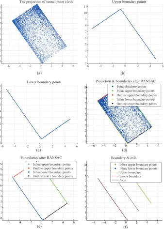
Figure 2.The sketch of every single step in tunnel axis acquisition. (a) is the projection of compressed
tunnel point cloud in the plane XOY. (b) illustrates the upper points extracted from every point cloud interval from xmin to xmax. (c) illustrates the lower boundary points extracted from every point cloud interval from xmin to xmax. (d) illustrates the point cloud projection and all boundaries including inline and outline upper boundaries and inline and outline lower boundaries fitted through the points extracted in (b) and (c) after RANSAC. (e) illustrates all boundaries fitted through boundary points after RANSAC. (f) extract the inline upper, lower boundaries and axis extracted from inline boundaries.
2.3. Tunnel point clouds segments extraction
The tunnel structures in cities, shield tunnels, pipe-jacking tunnel or other circular tunnels, are mainly constituted of concrete tunnel linings or tunnel tubes. On the other hand, the radial deformation of tunnel primarily occurs in tunnel segment joints with the result that the stiffness of joints is smaller than that of the tunnel segment. So the monitoring based on TLS of radial deformation should mainly focus on the tunnel segments[50]. Therefore, it’s meaningful to segment tunnel point clouds and extract the segment to analyze the radial deformation of tunnel.
In order to simply the process and improve the efficiency on the premise of sufficient accuracy, the segment extraction module applies the method that divides the tunnel point clouds into small parts equally to extract point cloud segments. The procedures of tunnel point clouds segment extraction are as follows:
1. Cut out a section of tunnel point clouds withnlinings and axis with equal length axis acquired in Section 2.2.m;
2. Divide the axis of the selected tunnel point clouds intonsegments equally and get n-1 equal diversion points in the axis;
3. Divide the selected tunnel point clouds with known number of linings by the normal planes in equal diversion points intonsegments then the tunnel point clouds segments extraction finish; 4. Extract the tunnel point cloud segments between two adjacent normal planes and then the tunnel
point clouds segments extraction finish.
(a) (d) (b) (c) 3 5 0 -5 0 2 4 6 8 10 -2 -1 0 1 2
A segment of tunnel point cloud -1 0 1 2 4 2 0
Point cloud & axis
-2
-4 2 0
4 6 8 10 -1 0 1 2 4 2 0
Point cloud & axis with equidistant points
-2
-4 2 0
4 6 8 10 0 1 2 3 4 44 42 40
A segment of tunnel point cloud
38 36 -50 -48 -46 -44 -42 -40
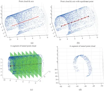
Figure 3.The procedure of tunnel point clouds segments extraction. (a) illustrates the tunnel point
clouds with axis. (b) illustrates the equal diversion in the axis of a section of tunnel point clouds. (c) illustrates that the normal planes in equal diversion points divide the tunnel point clouds into lining segments. (d) illustrates the tunnel point cloud segment used for subsequent data processing.
2.4. Denoising of point clouds data
Various errors and noises exist in the acquired data and denoising is thus very essential. In general, the point clouds scanned by TLS in tunnel consist of parts of points reflected by the surface of the facility and equipment in the tunnel and this part of data is useless for subsequent data processing. Besides, noise is generated in point clouds data because of other human factors and environmental factors such as dust in tunnel, high reflective surface and miss operation. In a word, the noise should be removed to minimize its influence on the subsequent processing operations.
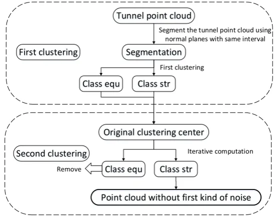
The proposed algorithm contains a special module based on clustering for noise removal with main focus on the redundant point clouds caused by the equipment and facilities in the tunnel. The raw point clouds of the structure contain mainly two kinds of noise: the first kind of noise is generated as a result of existence of facilities and equipment in the tunnel; the second kind of noise is generated due to the unusual reflectivity of scanned surface, generally light-reflecting and light-absorption surface. The first kind of noise is obvious and it is necessary to eliminate it or the data processing can’t continue. The second kind of noise has a negative effect on the result accuracy and is difficult to locate and distinguish because the noise distributes in point clouds randomly. The cost of removal of the second kind of noise is fairly high. So the second kind of noise is eliminated in the follow processor which is based on RANSAC algorithm.
are in direct contact with the tunnel lining so that the difference of distance is too small to cluster. In conclusion, it’s hard to eliminate the point clouds generated by the facilities efficiently and accurately. On the other hand, the LiDAR intensity is based on the optical strength which highly depends on the reflectance properties of the scanned materials [51]. So different materials may reflect laser beams with different intensity strengths even with an equal distance and incidence angle. The facilities and equipment in the tunnel are generally made of metal and rubber or the surface is covered with paint, which is totally different from the concrete tunnel lining surface with respect of reflectance properties. The proposed algorithm employs the second clustering based on intensity at the outcome of clustering based on distance to assist the analysis and improve the accuracy. The flowchart of the proposed algorithm is illustrated by Fig. 4.
Tunnel point cloud
Segmentation
Segment the tunnel point cloud using normal planes with same interval
Class str
Original clustering center
Point cloud without first kind of noise First clustering
Iterative computation
Remove
Class equ
Class str Class equ
First clustering
Second clustering
Figure 4.Flow chart of proposed algorithm based on twice clustering based on distance and intensity
orderly to denoise
The first clustering based on distance:
1. Avoid clustering of the whole structure point clouds at a time and segment the tunnel point clouds so the clustering analysis can be implemented in every segment extracted in section 2.2.3, which can reduce complexity and computing time of the algorithm and improve the stability of the algorithm while assuring accuracy;
2. Normalize the coordinates of axis and tunnel point clouds segment. Transfer the tunnel point cloud segment by coordinate transformation matrix to where the tunnel axis is coincident with designed coordinate axis;
3. Cluster the tunnel point clouds based on distance. A supervised algorithm is applied to label points of classes: str stands for point clouds rejected by the structure and equ represent point clouds from facilities and equipment once point clouds are clustered. Calculate the distance between every single point in point clouds and the tunnel axis and then set threshold values R+∆randR−∆rcorresponding to class str and class equ respectively, whereRis the radius of the tunnel and∆ris the threshold of distance.
the points reflected by facilities and equipment only. However, the class str may also contain part of equipment point clouds and is implemented twice in clustering analysis based on intensity later.
(a) (b) 0 1 2 3 4 44 42
Raw data with distance to axis
40 38
36 -40 -42 -44 -46 -48 -50
1.4 1.6 1.8 2 2.2 2.4 2.6 2.8 Distance(m) Distance(m) 0 1 2 3 4 5 6 7 8 9 10
Number of points
×104 Distance to axis distribution of the point cloud
3.5 3 2.5 2 1.5 1
Figure 5.Distance distribution of raw point clouds in experiments
Tunnel point clouds contain massive data information which results in huge time-consumption. Setωas dilution factor applied in uniform sampling of the massive data to reduce the computational
time.
NA=ω·Ni (6)
WhereNiis the number of points in segmentiandωis the dilution factor defined by the amount
of data and requirement of algorithm efficiency,NAis the actual point number in calculation.
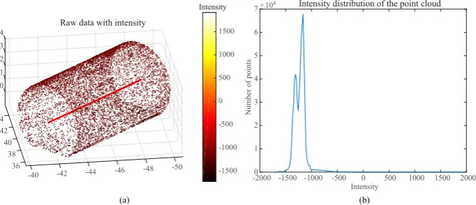
The second clustering analysis is based on intensity and is implemented on the result of the first clustering analysis. Akca suggested that intensity values can supply decent additional information for identification [52]. Fig. 6 denotes the intensities distribution of point cloud in experiments. It’s obvious that most of points concentrate in the area around value -1500 to -1000.
(a) (b) 0 1 2 3 4 44 42
Raw data with intensity
40 38
36 -40 -42 -44 -46 -48 -50 -1500 -1000 -500 0 500 1000 1500 Intensity
-2000 -1500 -1000 -500 0 500 1000 1500 2000 Intensity 0 1 2 3 4 5 6 7
Number of points
×104 Intensity distribution of the point cloud
Figure 6.Intensity distribution of raw point clouds in experiments
The second clustering uses the labeled points as training samples to set up pattern statistics like mean and variance of the cluster properties such as value of intensity for the two classes:
1. Obtain the original clustering center of the two classes str and equ from the result of first clustering analysis:
C0[C] = ∑
j∈C
Ij
WhereC0is the initial clustering center,IJis the intensity value,Crepresents class str or class equ
andNcis the total point number of class str or class equ;
2. Calculate the distance between every residual point and two initial clustering centers and cluster the points to the nearest class. Then recalculate the clustering centers of the two classes:
Ck[C] =
∑
j∈C
Ij
NC (8)
Wherekis the iterations;
3. The iterative calculation ends when the difference between a new clustering center and last clustering center is equal to or less than the threshold.
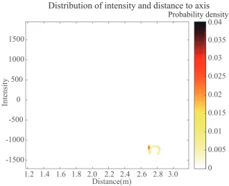
Through the verification by experiments, the proposed denoising algorithm can remove the point clouds reflected by facilities and equipment efficiently and accurately. Fig. 7 illustrates the two-dimensional probability distribution of distance and intensity of the proposed algorithm.
Distribution of intensity and distance to axis
1.2 1.4 1.6 1.8
2.2 2.4 2.6 2.8
Distance(m)
-1500
-1000
-500
0
500
1000
1500
Intensity
0
0.005
0.01
0.015
0.02
0.025
0.03
0.035
0.04
Probability density
3.0
2.0
Figure 7.Two-dimensional probability distribution of distances and intensities
2.5. Extraction of circle tunnel deformation
The proposed monitoring system based on TLS can make full use of massive spatial data acquired by the scanner and also deepen our cognition of structure state greatly. This chapter digs deeper into the tunnel point clouds segments to get more comprehensive information of tunnel’s structural health.
According to the existing researches and engineering experiences, tunnel deformation is one of the most direct indicators used to analyze the tunnel condition [53] [54]. So the proposed processing method chooses the radial deformation as the monitor indicator to reflect the safety condition of tunnel structure. Timothy et al. [18] calculated the algebraic deviations and mean absolute error and root mean square error between the measured radius value and the design radius to assess the condition of tunnels.
structure in operation gets deformed before failure under the nonuniform stress from surrounding stratums and can be approximately treated as an ellipse with tiny difference between long axis and minor axis. Hereby, the ovality and three-dimensional deformation nephogram are employed to indicate radial deformation of tunnel structure [55].
The processor employs the RANSAC algorithm for curve-fitting to acquire the ellipse of the tunnel cross-section formed by scanned points and analyze the radial deformation. The ovality is illustrated by the following formula whereTrepresents the tunnel ovality:
T= F− f
D (9)
WhereFis the length of long axis and f is the length of minor axis of ellipse fitted,Ris the design radial of tunnel. Fig 8 denotes the result of a tunnel point cloud segment produced by the proposed monitoring system.
−4 −3 −2 −1 0 1 2 3 4
−4 −3 −2 −1
0
1 2 3 4
0
30
60 90
120
150
180
210
240 270
300 330
Result of ellipse fitting Deformation in the long axis direction of the ellipse is 33mmDeformation in the short axis direction of the ellipse is −39mm Ovality is 1.32%
Amplify the deformation tenfold
0 30 60 90 120 150 180 210 240 270 300 330 360 −100
−80 −60 −40 −20
0
20 40
60
80 100
Angle
Deformation in radial direction
mm
Point cloud Standart circle Fitting ellipse
(a) (b)
Figure 8.The ovality of a tunnel point cloud segment produced by the proposed monitoring system.
(a) is the comparison between the ellipse fitted by point cloud and the standard circle which represents the designed schema. (b) is the unfolding drawing of (a) and illustrates a more intuitional comparison about deformation at different central angles.
0.20.71.2
−2 −1
0 1
2
−2
−1.5
−1
−0.5
0 0.5 1 1.5 2 2.5
The three−dimensional deformation nephogram
Deflection(mm)
−40 −30 −20 −10
0 10 20
30 40
50 60
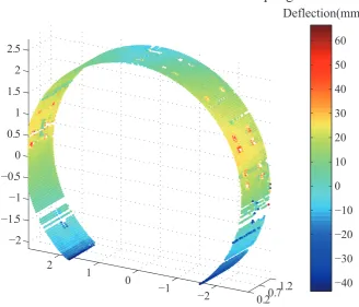
Figure 9.The three-dimensional deformation nephogram of a single tunnel point clouds segment. The
different values of deformation are expressed by different colors.
The ovality and three-dimensional deformation nephogram can make full use of the massive information contained in point clouds collected by TLS and demonstrate the deformation of almost every point in a tunnel to reflect its health condition.
3. Error analysis
Errors of the proposed processing method mainly consist of single point location error, measuring error and algorithm error[55]. The single point location error is defined by the accuracy of scanner hardware. The TLS point clouds data were acquired from the Leica Scanstation C10 and measurements taken with this type of laser scanner resulted in range precision of 4 mm and range distance 134 m @ 90% reflectivity. The measuring error can be restricted within the permissible range efficiently by adjusting the distance between two adjacent stations and incidence angle. The algorithm error occurs as a result of some unavoidable limitations of algorithm can transmit and amplify the deviation and is difficult to evaluate[56][57][58][59].
An operation is simulated to analyze the error produced in the proposed monitoring system, a conventional monitoring system based on total station is applied for subsidiary and the surveying result is compared to quantify the error and obtain the realistic accuracy of the proposed processing method.
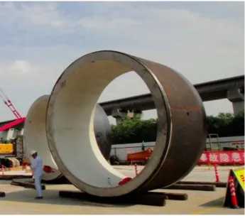
Figure 10.The pipe-jacking tunnel lining used in the experiment
Table 1. The instrument parameters of the laser scanner and total station used in two monitoring
systems
Total station Laser scanner
Name Leica TS30 Leica C10
Angle accuracy 0.5" 12"
Range accuracy 2mm+2ppm 4mm(50m)
3 -3 -2 -1 0 1 2 3 -3 -2 -1 0 1 2 3 -3 -2 -1 0 1 2 3 -3 -2 -1 0 1 2 -3 -2 -1 0 1 2 3 -3 -2 -1 0 1 2 3 90° 300 270 ° 240° 210° 180° 150°
120° 60°
30° 360° 330° ° 90° 300 270 ° 240° 210° 180° 150°
120° 60°
30° 360° 330° ° 90° 300 270 ° 240° 210° 180° 150°
120° 60°
30°
360°
330°
°
Amplify the deformation tenfold Amplify the deformation tenfold Amplify the deformation tenfold
(a) (b) (c)
Figure 11.The profiles fitted by the data acquired in the experiments. (a) denotes the profile fitted by
the first set of data collected by the total station; (b)denotes the profile fitted by the second set of data collected by the total station; (c) illustrates the profile fitted by the point cloud scanned by the TLS.
distance between the point with same central angle measured by total station and TLS in different measurements as measurement error of the proposed monitoring system and obtain the histograms (Fig. 12).
一
甀洀
戀攀
爀 漀
昀 瀀
漀椀
渀琀
猀
䴀攀愀猀甀爀攀 攀爀爀漀爀 ⠀洀洀⤀
밃㴀 ⸀洀洀 쌃㴀⸀㈀洀洀
一
甀洀
戀攀
爀 漀
昀 瀀
漀椀
渀琀
猀
䴀攀愀猀甀爀攀 攀爀爀漀爀 ⠀洀洀⤀
밃㴀 ⸀洀洀 쌃㴀⸀㈀洀洀
⠀愀⤀ ⠀戀⤀
Figure 12.Histograms of differences between measurements by TLS and two measurements of the
total station. (a) denotes the quantitative distribution of measurement error of the proposed monitoring system which takes the first set of data from total station as standard; (b) denotes the quantitative distribution of measurement error of the proposed monitoring system which takes the second set of data from total station as standard.
Input the measurements illustrated in Fig. 12 for statistical analysis through Jarque-Bera test, the measurement error shown in Fig. 12 left follows the normal distribution with mean value of 0.1mm and standard deviation of 1.2mm and the right also follows normal distribution with mean value of -0.1mm and standard deviation of 1.2mm.
4. Application
The proposed monitoring system is aimed at achieving automation and high efficiency of tunnel structure health monitoring within the permissible engineering range. This section describes application of the proposed processing method to a practical project and compares the efficiency of point cloud processing method the automatic way and the conventional manual way.
4.1. Practical monitoring project
Shanghai metro line 7 was put into operation in 2009 with a total length of approximately 44.35km, which is constructed with two side-by-side tunnels with an inner diameter of 5.5m by slurry balance shield. The tunnel is formed by lining segments loop by loop with a length of 1.2m and every single loop is assembled by six lining segments with one top block, one bottom block and four standard blocks.
Figure 13. The realistic picture and point cloud of Shanghai metro line 7 scanned by TLS in this monitoring project. There is a Leica C10 scanstation in tunnel
The geometric arrangement of scan stations is indicated by Fig. 14. Define the∆H(m) as the vertical distance from the scan station to the center of the tunnel and∆T(m) as the horizontal distance (Fig. 14 (a)).
A
B E
α α
A B
D C
Scan
station 1 Scanstation 2 station 3Scan
F F
E
max max Tunne
l diame
ter D
ΔL
ΔH
ΔT
ΔL
Figure 14.The geometric arrangement of scan station of TLS in circle tunnels. (a) illustrates the cross
section which contains pointsAandBin the right picture. (b) is the longitudinal section of tunnel and contains pointsAandBin the left picture.
4.2. Monitoring project efficiency analysis
The proposed processing method mainly focuses on automation of point cloud processing. The proposed processing method processes the massive data in a fully automatic way to significantly improve the efficiency of point cloud processing and allow the engineers to do other more meaningful work.
The steps of manual point clouds processing are as follows: first label the tunnel linings in a fixed direction for convenience of subsequent processing; then segment the tunnel point clouds; remove the obvious noise, namely, the points reflected by the facilities and equipment inside the tunnel; implement ellipse-fitting for tunnel segment point clouds through business software to extract the axis; finally export the processed information. As to subway tunnel, the time consumed in processing a single tunnel lining point cloud segment is about 6 minutes according to experience.
The monitored zone contains 100 tunnel lining segments and the 3D point clouds data scanned in the zone is processed by conventional method and the proposed method separately, by the same computer. Tab. 2 denotes the difference between results of the two methods.
Table 2.Comparison in post-processing time between two methods
The proposed monitoring system Conventional manual way
Steps Times/second Steps Times/second
Axis acquisition 30 Label linings 5000
Segments extraction 2.5 Segments extraction 6500
Denoising 17.5 Denoising 8000
Axis extraction 10000
Error correction 5000
According to the comparison from the above table, the largest component of computational time consumed in the conventional method is the manual noise removal, lining segment division and tunnel axis extraction. These manual operations are not only time-consuming but also affect accuracy adversely.
The conventional method of point cloud processing mainly depends on manual operations and business software, which is a time-consuming and labor intensive work with low accuracy. The business software is designed for all customers in various industries, so most of the functions are universal and not specially designed for tunnel point clouds processing. The manual extraction of tunnel lining segments cannot provide precise measurements due to manual partition of tunnel point clouds which totally depends on the difference in joint intensity with naked eye. The manual removal of obvious noise reflected by facilities inside the tunnel is very cursory because the selection tool in Cyclone (business software applied for raw point clouds data processing of Leica) is fixed and it does not suit the geometry of tunnel point clouds. On the other hand, the defects in manual removal of noise also result in over denoising or inadequate denoising.
No. 386
No.420
No.450
21point cloud1.221.51.41.81.61.81.621.41.211-40-30-20-10010203040deflection(mm)
2 1
point cloud
1.2
2 1.5
1.4
1.8 1.6 1.8
1.6 2
1.4 1.2 1
1 -40
-30 -20 -10 0 10 20 30 40
deflection(mm) Deflection (mm)
Figure 15.The overall deformation nephogram of the Shanghai metro line 7
5. Conclusions
This article proposes an automatic circle tunnel point cloud processing method based on 3D LiDAR data that extracts the tunnel deformation through ovality and a three-dimensional nephogram.
The proposed processing method puts forward a series of efficient and accurate algorithms to automatically process point clouds of circle tunnel. Firstly it extracts the tunnel axis using algorithms based on RANSAC; then extracts tunnel segments from the entire tunnel point clouds precisely by equally dividing the axis; next removes the obvious noise by twice clustering; finally obtains the ovality and tunnel deformation nephogram for evaluation of circle tunnel radial deformation.
The proposed monitoring system mainly focuses on circle tunnels. According to the analysis of the field contrast test and practical application in Shanghai metro line 7, the proposed processing method significantly improves the efficiency of point cloud processing within the engineering permissible range. The indicators employed in result analysis especially nephogram obtain more abundant reference information for the evaluation of tunnel structure and can fully develop the advantage of massive information from 3D LiDAR clouds.
Author Contributions:X. Xie conceived and designed this work. M. Zhao and J. He implemented the acquisition
system, analyzed the data and wrote the computer programs. X. Xie instructed M. Zhao to write the manuscript. X. Xie and B. Zhou revised the work. All the authors have approved the submitted version of the manuscript, have agreed to be personally accountable for their own contributions and for ensuring that questions related to the accuracy or integrity of any part of the work, are appropriately investigated, resolved, and documented in the literature.
Funding:This research was funded by National Nature Science Founds of China (51778476, 51608379), Shanghai
Science and Technology Development Funds (16DZ1200402, 17DZ1204203), and Guangxi Science and Technology Development Funds (2015BC17047).
Conflicts of Interest:The authors declare no conflict of interest.The founding sponsors had no role in the design
of the study; in the collection, analyses, or interpretation of data; in the writing of the manuscript, and in the decision to publish the results.
References
1. B. Riveiro, M.J. DeJong, B. Conde. Automated processing of large point clouds for structural health monitoring of masonry arch bridges.Automation in Construction2016,72, 258-268.
2. Hu, Shaoxing and Chen, Chunpeng and Zhang, Aiwu and Sun, WD, Zhu, Linlin. A Small and Lightweight Autonomous Laser Mapping System without GPS.Journal of Field Robotics2013,30, 784-802.
3. Kang Zhizhong, Zhang Liqiang, Tuo Lei, Wang Baoqian, Chen Jinlei. Continuous Extraction of Subway Tunnel Cross Sections Based on Terrestrial Point Clouds.Remote Sensing2013,6, 857-879.
4. Stephanie Fekete, Mark Diederichs. Integration of three-dimensional laser scanning with discontinuum modelling for stability analysis of tunnels in blocky rockmasses.International Journal of Rock Mechanics and
5. L. Díaz-Vilariño, H. González-Jorge, M. Bueno, P. Arias, I. Puente. Automatic classification of urban pavements using mobile LiDAR data and roughness descriptors.Construction and Building Materials2016,
102, 208-215.
6. Jongsuk Yoon, Myung Sagong, J.S. Lee, Kyusung Lee. Feature extraction of a concrete tunnel liner from 3D laser scanning data.NDT & E International2009,42, 97-105.
7. Mani Golparvar-Fard, Jeffrey Bohn, Jochen Teizer, Silvio Savarese, Feniosky Peña-Mora. Evaluation of image-based modeling and laser scanning accuracy for emerging automated performance monitoring techniques.Automation in Construction2011,20, 1143-1155.
8. Son Hyojoo, Kim Changwan. Automatic segmentation and 3D modeling of pipelines into constituent parts from laser-scan data of the built environment.Automation in Construction2016,68, 203-211.
9. Abellan Antonio, Vilaplana Joan, Calvet Jaume, Rodriguez-Lloveras Xavier. Detection of precursory deformation using a TLS.Natural Hazards and Earth System Sciences2009,9, 365-372.
10. Stephanie Fekete, Mark Diederichs, Matthew Lato. Geotechnical and operational applications for
3-dimensional laser scanning in drill and blast tunnels.Tunnelling and Underground Space Technology2010,25, 614-628.
11. Yusuf Arayici. An approach for real world data modelling with the 3D terrestrial laser scanner for built environment.Automation in Construction2007,16, 816-829.
12. Cai Hubo, Rasdorf William. Modeling Road Centerlines and Predicting Lengths in 3-D Using LIDAR Point Cloud and Planimetric Road Centerline Data.Comp.-Aided Civil and Infrastruct. Engineering.2008,23, 157-173. 13. Park H.S., Lee H.M., Adeli Hojjat, Lee Impyeong. A New Approach for Health Monitoring of Structures:
Terrestrial Laser Scanning.Comp.-Aided Civil and Infrastruct. Engineering.2007,22, 19-30.
14. Yan Yiming, Tan Zhichao, Su Nan, Zhao Chunhui. Building Extraction Based on an Optimized Stacked Sparse Autoencoder of Structure and Training Samples Using LIDAR DSM and Optical Images.Sensors 2017,17, 1957.
15. Morsy Salem, Shaker Ahmed, El-Rabbany Ahmed. Multispectral LiDAR Data for Land Cover Classification of Urban Areas.Sensors2017,17, 958.
16. Jung Jaewook, Jwa Yoonseok, Sohn Gunho. Implicit Regularization for Reconstructing 3D Building Rooftop Models Using Airborne LiDAR Data.Sensors2017,17, 621.
17. Choi Dong-Geol, Bok Yunsu, Kim Jun-Sik, Shim Inwook, Kweon Inso. Structure-From-Motion in 3D Space Using 2D Lidars.Sensors2017,17, 242.
18. Timothy Nuttens, Cornelis Stal, Hans De Backer, Ken Schotte, Philippe Van Bogaert, Alain De Wulf. Methodology for the ovalization monitoring of newly built circular train tunnels based on laser scanning: Liefkenshoek Rail Link (Belgium).Automation in Construction2014,43, 1-9.
19. Jen-Yu Han, Jenny Guo, Yi-Syuan Jiang. Monitoring tunnel profile by means of multi-epoch dispersed 3-D LiDAR point clouds.Tunnelling and Underground Space Technology2013,33, 186-192.
20. Jen-Yu Han, Jenny Guo, Yi-Syuan Jiang. Monitoring tunnel deformations by means of multi-epoch dispersed 3D LiDAR point clouds: An improved approach. Tunnelling and Underground Space Technology2013,38, 385-389.
21. Borja Rodríguez-Cuenca, Silverio García-Cortés, Celestino Ordóñez, Maria C. Alonso. An approach to detect and delineate street curbs from MLS 3D point cloud data.Automation in Construction2015,51, 103-112. 22. Andrey Dimitrov, Mani Golparvar-Fard. Segmentation of building point cloud models including detailed
architectural/structural features and MEP systems.Automation in Construction2015,51, 32-45.
23. Frédéric Bosché, Mahmoud Ahmed, Yelda Turkan, Carl T. Haas, Ralph Haas. The value of integrating Scan-to-BIM and Scan-vs-BIM techniques for construction monitoring using laser scanning and BIM: The case of cylindrical MEP components.Automation in Construction2015,49, 201-213.
24. F. Bosche, C.T. Haas. Automated retrieval of 3D CAD model objects in construction range images.Automation
in Construction2008,17, 499-512.
25. ebekka Volk, Julian Stengel, Frank Schultmann. Building Information Modeling (BIM) for existing buildings — Literature review and future needs.Automation in Construction2014,38, 109-127.
26. Pingbo Tang, Burcu Akinci, Daniel Huber. Quantification of edge loss of laser scanned data at spatial discontinuities.Automation in Construction2009,18, 1070-1083.
28. J. Jaselskis Edward, Gao Zhili, C. Walters Russell. Improving Transportation Projects Using Laser Scanning.
Journal of Construction Engineering and Management2005,131, 377-384.
29. C. Cabo, S. García Cortés, C. Ordoñez. Mobile Laser Scanner data for automatic surface detection based on line arrangement.Automation in Constructio2015,58, 28-37.
30. Kukko Antero, Kaartinen Harri, Hyyppä Juha, Chen Yuwei. Multiplatform Mobile Laser Scanning: Usability and Performance.Sensors2012,12, 11712-33.
31. Castaño Fernando, Beruvides Gerardo, Haber Guerra Rodolfo Elias, Artuñedo Antonio. Obstacle Recognition Based on Machine Learning for On-Chip LiDAR Sensors in a Cyber-Physical System.Sensors2017,17, 2109.
32. Meng Xiaoli, Wang Heng, Liu Bingbing. A robust vehicle localization approach based on
GNSS/IMU/DMI/LiDAR sensor fusion for autonomous vehicles.Sensors2017,17, 2140.
33. Oh Sang-Il, Kang Hang-Bong. Object Detection and Classification by Decision-Level Fusion for Intelligent Vehicle Systems.Sensors2017,17, 207.
34. Kim Jung-Un, Kang Hang-Bong. A new 3D object pose detection method using LIDAR shape set.Sensors 2018,18, 882.
35. I. Puente, H. González-Jorge, J. Martínez-Sánchez, P. Arias. Review of mobile mapping and surveying technologies.Measurement2013,46, 2127-2145.
36. Iván Puente, Higinio González-Jorge, Joaquín Martínez-Sánchez, Pedro Arias. Automatic detection of road tunnel luminaires using a mobile LiDAR system.Measurement2014,47, 569-575.
37. Alireza G. Kashani, Andrew J. Graettinger. Cluster-Based Roof Covering Damage Detection in Ground-Based Lidar Data.Automation in Construction2015,58, 19-27.
38. G. Kashani Alireza, Olsen Michael, Graettinger Andrew. Laser Scanning Intensity Analysis for Automated Building Wind Damage Detection.Congress on Computing in Civil Engineering, Proceedings2015, 199-205. 39. Han Jen-Yu, Chen Chuin-Shan, Lo C.T. Time-Variant Registration of Point Clouds Acquired by a Mobile
Mapping System.IEEE Geoscience and Remote Sensing Letters2014,11, 196-199.
40. Yan Li, Tan Junxiang, Liu Hua, Xie Hong, Chen Changjun. Automatic Registration of TLS-TLS and TLS-MLS Point Clouds Using a Genetic Algorithm.Sensors2017,17, 1979.
41. Michele Fumarola, Ronald Poelman. Generating virtual environments of real world facilities: Discussing four different approaches.Automation in Construction2011,20, 263-269.
42. P.J. Besl, N.D. McKay. A method for registration of 3-D shapes.IEEE Transactions on Pattern Analysis and
Machine Intelligence1992,14, 239-256.
43. Chen Yang, Medioni Gérard. Object Modeling by Registration of Multiple Range Images. Image Vision
Comput.1992,10, 145-155.
44. Zhang Zhengyou. Iterative point matching for registration of free-form curves and surfaces.International
Journal of Computer Vision1994,13, 119-152.
45. Wang Zhi, Brenner Claus. Point based registration of terrestrial laser data using intensity and geometry features. International Archives of Photogrammetry, Remote Sensing and Spatial Information Sciences2008,
XXXVII(B5), Beijing, China, 583–589.
46. Wang Baoqian, Kang Zhizhong. Self-closure global registration for subway tunnel point clouds.Proceedings
of International Conference on Computer Vision in Remote Sensing2012, 152-157.
47. Han Soohee, Cho Hyungsig, Kim Sangmin, Jung Jaehoon, Heo Joon. Automated and Efficient Method for Extraction of Tunnel Cross Sections Using Terrestrial Laser Scanned Data. Journal of Computing in Civil Engineering.Journal of Computing in Civil Engineering2013,27, 274-281.
48. Plaza-Leiva Victoria, Antonio Gomez-Ruiz Jose, Mandow Anthony, Garcia Alfonso. Voxel-Based
Neighborhood for Spatial Shape Pattern Classification of Lidar Point Clouds with Supervised Learning.
Sensors2017,17, 594.
49. Fischler M A, Bolles R C. Random sample consensus: a paradigm for model fitting with applications to image analysis and automated cartography.Commun. ACM1981,24, 381-395.
50. Maalek R, Lichti D D, Ruwanpura J Y. Robust Segmentation of Planar and Linear Features of Terrestrial Laser Scanner Point Clouds Acquired from Construction Sites.Sensors2018,18, 819.
51. Pfeifer Norbert, Dorninger Peter, Haring Alexander, Fan Hongchao. Investigating terrestrial laser scanning intensity data: quality and functional relations.International Conference on In: Gruen2006.
52. Devrim Akca. Matching of 3D surfaces and their intensities.ISPRS Journal of Photogrammetry and Remote
53. M. Lewis Gregory, H Austin Philip, Szczodrak Malgorzata. Spatial statistics of marine boundary layer clouds.J. Geophys. Res.2004,109.
54. Hu Qingwu, Wanling Yin. Tempo-space Deformation Detection of Subway Tunnel based on Sequence
Temporal 3D Point Cloud.Disaster Advances2012,5, 1326-1330.
55. Li Xiaolu, Yang Bingwei, Xie Xinhao, Li Duan, Xu Lijun. Influence of Waveform Characteristics on LiDAR Ranging Accuracy and Precision.Sensors2018,18, 1156.
56. Zeng Yadan, Yu Heng, Dai Houde, Song Shuang, Lin Mingqiang, Sun Bo, Jiang Wei, Q-H Meng Max. An improved calibration method for a rotating 2D LIDAR system.Sensors2018,18, 497.
57. Morales J, Plaza-Leiva Victoria, Mandow Anthony, Antonio Gomez-Ruiz Jose, Serón Javier, Garcia Alfonso. Analysis of 3D Scan Measurement Distribution with Application to a Multi-Beam Lidar on a Rotating Platform.Sensors2018,18, 395.
58. Li Xiaolu, Wang Hongming, Yang Bingwei, Huyan Jiayue, Xu Lijun. Influence of Time-Pickoff Circuit Parameters on LiDAR Range Precisione.Sensors2017,17, 2369.
59. Gao Z., Lao M., Sang Y., Wen F., Ramesh B., Zhai R. Fast Sparse Coding for Range Data Denoising with Sparse Ridges Constraint.Sensors2018,18, 1449.
60. Kaasalainen Sanna, Jaakkola Anttoni, Kaasalainen Mikko, Krooks Anssi, Kukko Antero. Analysis of Incidence Angle and Distance Effects on Terrestrial Laser Scanner Intensity: Search for Correction Methods.
Remote Sensing2011,3, 2207-2221.
61. Ramón Argüelles-Fraga, Celestino Ordóñez, Silverio García-Cortés, Javier Roca-Pardiñas. Measurement planning for circular cross-section tunnels using terrestrial laser scanning.Automation in Construction2013,
31, 1-9.
62. Yang Ronghua, Hua X, Qiu W, Tang K, Geng T. Terrestrial laser scanners’s angular resolution of any direction.
Journal of Geomatics2011,36, 11-12+54.
63. Pingbo Tang, Daniel Huber, Burcu Akinci, Robert Lipman, Alan Lytle. Automatic reconstruction of as-built building information models from laser-scanned point clouds: A review of related techniques.Automation in
Construction2010,19, 829-843.
64. Javier Roca-Pardiñas, Ramón Argüelles-Fraga, Francisco de Asís López, Celestino Ordóñez. Analysis of the influence of range and angle of incidence of terrestrial laser scanning measurements on tunnel inspection.
Tunnelling and Underground Space Technology2014,43, 133-13.
65. Marko Peji´c. Design and optimisation of laser scanning for tunnels geometry inspection. Tunnelling and
Underground Space Technology2013,37, 199-206.
66. Sylvie Soudarissanane, Roderik Lindenbergh, Massimo Menenti, Peter Teunissen. Scanning geometry: Influencing factor on the quality of terrestrial laser scanning points.ISPRS Journal of Photogrammetry and
Remote Sensing2011,66, 389-399.