Article
1
PAVEMENT DAMAGE CRACK RECOGNITION
2
METHOD BASED ON HIGH-RESOLUTION
3
LINEAR ARRAY CAMERAS AND ADAPTIVE
4
LIFTING ALGORITHM
5
Yi Han 1,*, Shiwei Tu 1, Yanyu Yang 1, Ke Lei 2and Chunlei Liu 3
6
1 School of Automobile, Chang’an University, Xi’an 710064, China; [email protected]
7
2 Shangtai Software (Shanghai) Co., Ltd., Shanghai 200020, China; [email protected]
8
3 Department of Computer Science, Valdosta State University, Valdosta 31698, USA ; [email protected]
9
* Correspondence: [email protected]; Tel.: +86-29-82334143
10
11
Abstract: This paper proposes a crack recognition method based on high-resolution line array
12
cameras and adaptive lifting algorithm. By defining the crack rate, this algorithm calculates the
13
ratio of the crack area to the area of the entire collected image to characterize the damage extent of
14
the current section. The algorithm first uses image preprocessing to reduce the image noise, then
15
uses histogram equalization to enhance the feature of the crack region, divides the whole image
16
into multiple sub-blocks, and extracts region features in the sub-block. At the same time, this
17
algorithm defines related feature descriptors, and constructs weak classifiers according to each
18
feature descriptor, and converts the weak classifiers into strong classifiers by using an adaptive
19
lifting algorithm. Finally, this algorithm realizes the division of the crack regions. Experimental
20
results show that the proposed algorithm can meet the actual needs and is better than other
21
classical algorithms.
22
Keywords: line array cameras; pavement crack detection; feature analysis; adaptive lifting
23
24
1. Introduction
25
With the large-scale construction of high-grade pavement in China in recent years, the
26
detection of pavement damage has become a very important task [1-4]. Currently, semi-automated
27
testing vehicle equipment is widely adopted in the detection of pavement problems. This approach
28
requires manual processing of offline data and fails to achieve full automatic detection of pavement
29
damage [5-6].It also has many obvious drawbacks. Firstly, the results of manual processing may be
30
affected by the subjectivity of manual detection and thus may not accurately and objectively reflect
31
the real conditions of pavement [7-8]. Secondly, the efficiency of manual detection is usually very
32
low, therefore consumes a lot of manpower. These drawbacks are extremely unfavorable to
33
highway management and maintenance. Moreover, the recognition effect of automatic
34
identification system is not satisfactory and there are still many problems [9-13]. The main causes of
35
these problems are: (1) pavement interference factors, such as shading shadows, water stains,
36
grease and so on; (2) complex road conditions, the lighting conditions of the pavement are different
37
at different time periods, which is highly detrimental to our identification; (3) pavement damage
38
types, including transverse cracks, longitudinal cracks, chaps, block fractures, etc.. In view of the
39
current testing needs and situation, this paper proposes the use of image processing technology,
40
combined with the adaptive lifting algorithm in machine learning to automatically identify the
41
crack area on the road image [14-18]. The algorithm has high recognition rate and fast speed, and
42
meanwhile can basically meet the actual needs.
43
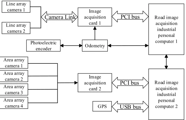
2. Materials and Methods
44
2.1. Image Acquisition
45
In this paper, high-resolution linear array cameras, image capture cards, combined with
46
integrated LED lights, industrial personal computer(IPC), optical encoder, GPS and other auxiliary
47
devices are used to acquire and store real-time road images, and are integrated as a whole system in
48
a commercial vehicle [19-22]. By contrast, we use line frequency of 140kHz, a resolution of 4k, the
49
model for the Basler sprint-spL4096-140km CMOS linear array cameras to capture road images
50
[23-26].
51
During the driving process of the vehicle, the photoelectric encoder rotates synchronously with
52
the wheel to generate TTL(Transistor-Transistor Logic) pulse signals, which are processed by the
53
data acquisition card and part of peripheral circuits [27-29]. The computer counts the pulses and
54
converts them into mileage and speed information in real time. In this process, the pulse generated
55
by the photoelectric encoder is modulated to generate a pulse trigger signal for the linear array
56
cameras. When the left and right linear array cameras are triggered, the image of the road surface is
57
collected [30-31]. After the image signal is processed by the image capture card via the Camera Link
58
interface, the image is transmitted to IPC memory to complete the acquisition and storage of
59
information on the road.
60
Line array
camera 1 Image acquisition
card 1
PCI bus Camera Link
USB bus PCI bus
Road image acquisition industrial
personal computer 1 Photoelectric
encoder Odometry
GPS Line array
camera 2
Area array camera 1 Area array
camera 2 Area array
camera 3 Area array
camera 4
Image acquisition
card 2
Road image acquisition industrial
personal computer 2
61
Figure 1. Image acquisition structure block diagram
62
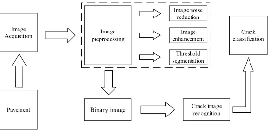
Pavement Image Acquisition
Crack image recognition
Crack classification
Binary image Image preprocessing
Image noise reduction
Image enhancement
Threshold segmentation
64
Figure 2. Operation flow chart
65
2.2. Image preprocessing
66
Before cracks in the captured image are identified, the image needs to be preprocessed because
67
acquisition hardware and the natural lighting in the actual scene may inevitably introduce some
68
interference and noise into the captured image [32-34]. In order to facilitate subsequent image
69
processing, these unfavorable factors must be eliminated firstly. To avoid the obvious shortcoming
70
of blurred image of the mean filter, we use the Gauss filter to reduce the image noise [35-38]. Our
71
Gauss filter has a size of 5×5, and can be expressed as:
72
73
1
4
7
4
1
4 16 26 16 4
1
7 26 41 26 7
273
4 16 26 16 4
1
4
7
4
1
GS
F
=
(1)
74
The convolution of the Gauss filter and the original image
P
o produces the noise-reduced75
image
P
d [39].76
P
d= ⊗
P
oF
GS (2)77
After some noise is eliminated with the Gauss filter, the image can be further processed to
78
enhance regional characteristics of the cracks to be identified and to weaken background features of
79
the images [40]. The purpose of this process is to reduce the impact of the background information
80
on the later recognition while preserving most of the crack information. We implement the image
81
enhancement with histogram equalization, which converts the input image to hold the same pixel
82
value in each gray scale[41-45]. This method can significantly enhance the contrast of the image.
83
Assuming that the gray scale range of the captured image is
[
0,
L
−
1
]
, the approximate probability84
of gray scale
r
k can be calculated as:85
( )
k,
0,1,...,
1
k
n
p r
k
L
N
=
=
−
(3)
Where
n
k is for the number of pixels in the image with gray scaler
k,N
is for the sum of87
the numbers of all the pixels, and
L
is for the number of gray scaler
k. Gray scaler
k and the88
probability of appearance of gray scale
p r
( )
k can be expressed as the histogram of the original89
image [46].
90
For gray images, the method of the enhancement of histogram equalization can be expressed
91
as [47]:
92
0
( )
( )
0,0
1
=
−
≥
≤ <
−
rkk
k i
f r
p i
r
L
L
(4)93
Where
94
0
( )
(0
)
=
=
rk≤ <
k j
j
f r
u
j L
(5)95
1
0
0
(0
)
j L
j j
u
j L
u
L
−
=
≥
≤ <
<
(6)
96
( )(0
k≤ <
k)
f r
r
L
stands for the mapping relationship between the pre-enhancement image gray97
scale
r
k and the enhanced image gray scaler
k'
.98
By the following formula, the transformed gray scale allows the output histogram to be uniform
99
over the entire output gray scale range so that the contrast of the image can be increased.
100
0
( )
k((
1)
k( ))
jj
T r
round L
p r
=
=
−
(7)
101
Figure 3 is a pavement crack image. After the image preprocessing, Figure 3 turns into Figure
102
4.
104
Figure 3. Original image
105
106
Figure 4. Image after preprocessing
107
Due to the complexity of the overall pavement condition, the gray value of cracks in different
108
regions of the image varies greatly. Even if the whole image is segmented by the noise reduction
109
with Gauss filter and the image enhancement with histogram equalization, the obtained results still
110
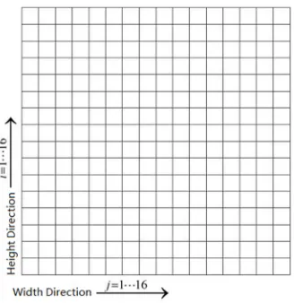
can't meet the actual needs. Therefore, we divide the whole image into a plurality of sub-blocks, and
111
the sub-block regions are separately subjected to threshold segmentation [48-49]. A collected 3024
112
× 2048 pavement image is divided into 16 × 16 blocks, as shown in Figure 5.
113
114
Figure 5. Regional block diagram
115
2.3. Feature selection
116
The 256 blocks fall into two categories, those containing cracks and those containing no cracks,
117
as shown in Figure 6.
119
Figure 6. Image after dividing into blocks
120
Observation and analysis of a large number of image samples reveal that the target of
121
pavement cracks has specific shape features that can be used to categorize the blocks. These shape
122
features can be obtained by binarizing the segmented image with the maximum entropy method.
123
The principle of maximum entropy method states that the entropy takes the maximum value when
124
all events of the system are equally likely to occur [50-51].
125
The following is the process to use the maximum entropy method to calculate the threshold.
126
For a gray image, assuming the range of the image gray values is
[0,
L
−
1]
, and the minimum and127
maximum gray values are
V
min andV
maxrespectively. According to the entropy formula, the128
entropy value corresponding to the gray value
t
can be calculated as129
( ) lg (1
)
1
t L t
t t
t t
H
H
H
E t
P
P
P
P
−
=
−
+
+
−
(8)130
Where
131
0
t
t i
i
P
p
=
=
(9)
132
0
lg
tt i i
i
H
p
p
=
= −
(10)
133
0
lg
LL i i
i
H
p
p
=
= −
(11)
134
Here
p
i is the probability that the gray valuei
appears,P
t is the sum of the probability of135
the gray values from 0 to
t
,H
t is the sum of the entropy of the gray values from 0 tot
, andH
L136
is the entropy of the original image. The objective of our method is to find a proper value of
t
137
between
V
min andV
max to maximizes E t( ). The value oft
is the optimal threshold determined138
by the maximum entropy method.
139
After the image process by using the threshold, there are still some discrete small particles in
140
the original picture. Therefore, four description values are designed as classification features of the
141
binary image for the obtained image area that is less than the threshold.
(1) The rectangularity of the largest connected region: the ratio of the area of the region to the
143
area of a rectangular region having the same first-order moment and second-order moment in this
144
region. For the fractured segment, the largest connected region is the region where the fractures are
145
located. And the rectangularity of the largest connected region of fractured segments is generally
146
smaller than the non-fractured segments.
147
(2) The eccentricity of the largest connected region: the ratio of the semi-major axis to the
148
semi-minor axis of the smallest ellipse that can cover the largest connected region. The larger the
149
ratio, the more likely there are cracks in the pavement image.
150
(3) The area of the largest connected region
151
max( )
=
iMA
A
(12)
152
where
A
i is the area of the ith connected domain.153
(4) The compactness of the largest connected region: the square of the length of the region
154
outline is divided by the area of the region.
155
2.4. Crack recognition classification
156
The regional characteristic descriptors obtained from the previous step can be used to
157
determine whether the current sub-block contains cracks. We utilize an adaptive lifting algorithm to
158
train the classifier to complete the related classification work [52]. The algorithm consists of the
159
following steps.
160
(1) Given
N
samples of the training data set, each sample contains the above four161
characteristic description values and whether it is a mark of a crack region or not. The sample set is
162
expressed as follows:
163
{ }
1 1 2 2
={(x ,y ),(x ,y ),...,(x ,y )};
N N1,1
T
y
= −
(13)
164
where
{ , }
x y
i i iN=1 stands for training sample set and the corresponding mark.165
(2) Initialize weights distribution of the training data set as
166
1 1,1 1, 1, 1,
1
(
,...,
i,...
N),
i,
1, 2,...
D
w
w
w
w
i
N
N
=
=
=
(14)
167
(3) For m =1, 2, 3, 4, uses a training dataset with weight distribution
D
m for learning, and168
generates the basic classifier
G x
m( )
[53]. In the meantime, calculates the error ratee
m of169
classification and the coefficient
α
m of the basic classifierG x
m( )
in the training data set using the170
following formulas.
, ( )
(
( )
)
m i i
m m i i m i
G x y
e
P G x
y
w
≠
=
≠
=
(15)
172
1
1
lg
2
m m
m
e
e
α
=
−
(16)
173
Where
w
m i, is the weight of the ith sample in roundm m
(
∈
{1, 2,3, 4})
, and174
, 1
1
N
m i i
w
=
=
(17)
175
(4) Update the distribution of weights of the training data set.
176
1
(
1,1,...,
1,,...,
1,)
m m m i m N
D
+=
w
+w
+w
+(18)
177
,
1,
exp(
( )),
1, 2...,
m i
m i m i m i
m
w
w
y G x
i
N
Z
α
+
=
−
=
(19)
178
Where
Z
m is the factor of normalization.179
, 1
exp(
( ))
N
m m i m i m i
i
Z
w
α
y G x
=
=
−
(20)
180
(5) Construct the linear combination of the basic classifier and obtain the strong classifier that
181
can determine whether the current sub-block image contains cracks.
182
4
1
( )
(
m m( ))
m
G x
sign
α
G x
=
=
(21)
183
The target area containing the cracks is marked with a red range. The damage rate is calculated
184
as the ratio of the number of marked sub-blocks to the total number of sub-blocks [54]. The
185
recognition results are shown in Figure 7.
186
188
(a)
189
190
191
(b)
192
194
(c)
195
Figure 7. Crack recognition results. (a) Transverse cracks; (b) Longitudinal cracks; (c) Irregular cracks
196
197
The overall algorithm is shown in Figure 8.
198
Noise reduction with Gauss filter
Image enhancement with histogram equalization
Image block
Image binarization with maximum entropy method
Classifier Adaptive lifting
algorithm
Whether the image contains cracks?
Mark the crack area Don't mark the
crack area
Determine the Crack type based on the image features
N
Y
199
Figure 8. Flow diagram of algorithm
200
201
3. Results
202
To verify the effectiveness of this algorithm, a set of 1000 pavement damage pictures provided
203
by a provincial highway bureau were used to perform a comparison experiment with manual
204
detection, and two other commonly used algorithms: the minimal deviation algorithm and the
205
OSTU algorithm. The experiment hardware environment is 2.40GHZ CPU, 8G memory IPC, and
206
the software environment is VC2010. The experiment was repeated eight times and the results are
207
shown below in Table 1.
208
209
Table 1. Average time taken to detect cracks in a single image by the four methods
Manual detection
Algorithm in this paper
Minimal deviation algorithm
OSTU algorithm
#1 4387ms 235ms 892ms 1233ms
#2 3315ms 346ms 1123ms 1452ms
#3 5789ms 532ms 965ms 1678ms
#4 4310ms 490ms 1387ms 1783ms
#5 3520ms 456ms 732ms 1653ms
#6 5120ms 378ms 1232ms 1723ms
#7 4760ms 612ms 934ms 1974ms
#8 4239ms 563ms 1365ms 1923ms
It can be seen that the detection speed of the algorithm in this paper is faster than that of
211
manual detection and the other two commonly used algorithms. We also compared the accuracy of
212
the detection methods of the four algorithms. The results are shown in Figure 9.
213
214
Figure 9. Accuracy of crack detection of the four methods
215
4. Discussion
216
From Figure 9, we can see that the accuracy of crack detection of the proposed algorithm is
217
slightly lower than manual detection, but far superior to the other two commonly used algorithms.
218
The accuracy of the algorithm in this paper can meet the detection accuracy requirements of the
219
actual pavement detection department.
220
5. Conclusions
221
Through theoretical research and actual experiments, we can draw the following conclusions:
222
(1) Currently, the detection of pavement crack is mainly conducted with manual identification.
223
On the other hand, there are still many problems with automatic recognition, such as slow
224
identification, poor accuracy and so on. Therefore, this paper adopts the adaptive lifting algorithm
225
for automatic pavement crack recognition.
226
0 0.2 0.4 0.6 0.8 1
1 2 3 4 5 6 7 8
Minimal deviation algorithm
Manual detection
Algorithm in this paper
(2) Through image processing combined with adaptive lifting model in machine learning, we
227
can calculate the ratio of the number of crack sub-blocks to the total number of image sub-blocks
228
and use it to characterize the degree of crack damage in the current image. The results suggest that
229
the speed and accuracy of recognition of our proposed algorithm can meet actual requirements.
230
(3) The current research mainly focuses on pavement cracks, but it cannot automatically detect
231
other types of damage, such as bags, pits, and repair of cracks. In the future, our research goal
232
should place on other types of damage pavement to further improve the automatic pavement
233
damage recognition system.
234
Acknowledgments: The Project Sponsored by the International Science and Technology Cooperation and
235
Exchange Projects of Shaanxi China (2016KW-063).
236
Author Contributions: Y.H. and C.L.L. conceived and designed the research; K.L., S.W.T. and Y.Y.Y.
237
performed the experiments; S.W.T. and Y.Y.Y. wrote the manuscript; Y.Y.Y. and S.W.T. analyzed the data;
238
C.L.L. and K.L. helped to design the comparison algorithm; and Y.H. helped to design image processing
239
methods.
240
Conflicts of Interest: The authors declare no conflict of interests.
241
References
242
243
244
1. Hasni, H.; Alavi, A.H.; Jiao, P.; Lajnef, N.; Chatti, K.; Aono,K.; Chakrabartty, S. A new approach for
245
damage detection in asphalt concrete pavements using battery-free wireless sensors with non-constant
246
injection rates, Measurement, 2017, 110, 217-229.
247
2. Zhang, D.; Li, Q.; Chen, Y.; Cao, M.; He, L.; Zhang B. An efficient and reliable coarse-to-fine approach for
248
asphalt pavement crack detection. Image and Vision Computing2017, 57, 130-146.
249
3. Ouma, Y.O.; Hahn, M. Pothole detection on asphalt pavements from 2D-colour pothole images using
250
fuzzy c-means clustering and morphological reconstruction. Automation in Construction2017, 83, 196-211.
251
4. Xu, X.; Peng, S.; Xia, Y.; Ji, W. The development of a multi-channel GPR system for roadbed damage
252
detection. Microelectronics Journal2014, 45, 1542-1555.
253
5. Kapela, R.; Śniatała, P.; Turkot, A.; Rybarczyk, A.; Pożarycki, A.; Rydzewski, P.; Wyczałek, M.; Błoch A.
254
Asphalt surfaced pavement cracks detection based on histograms of oriented gradients. 2015 22nd
255
International Conference Mixed Design of Integrated Circuits & Systems (MIXDES), Torun, 2015, pp.
256
579-584.
257
6. Li, J.; Zhang, Y.; Wang, L. Design and implementation of pavement crack detection system based on
258
FPGA. The 27th Chinese Control and Decision Conference (2015 CCDC), Qingdao, 2015, pp. 5936-5941.
259
7. Krysiński, L.; Sudyka J. GPR abilities in investigation of the pavement transversal cracks. Journal of
260
Applied Geophysics, 2013, 97, 27-36.
261
8. Hadjidemetriou, G.M.; Christodoulou, S.E.; Vela, P.A. Automated detection of pavement patches utilizing
262
support vector machine classification. 2016 18th Mediterranean Electrotechnical Conference (MELECON),
263
Lemesos, 2016, pp. 1-5.
264
9. Sun, L.; Qian, Z. Multi-scale wavelet transform filtering of non-uniform pavement surface image
265
background for automated pavement distress identification. Measurement, 2016, 86, 26-40.
266
10. Pereira, F.C.; Pereira, C.E. Embedded Image Processing Systems for Automatic Recognition of Cracks
267
11. Cheng, H.D.; Miyojim, M. Automatic pavement distress detection system. Information Sciences,1998, 108,
269
219-240,
270
12. Radopoulou, S.C.; Brilakis,I. Patch detection for pavement assessment. Automation in Construction, 2015,
271
53, 95-104,
272
13. María, V.G.; Mercedes, S.; Joaquín, M.S.;Arias, P. A semi-automatic processing and visualisation tool for
273
ground-penetrating radar pavement thickness data. Automation in Construction,2014, 45, 42-49.
274
14. Mataei, B.; Nejad, F.M.; Zahedi, M.; Zakeri, H. Evaluation of pavement surface drainage using an
275
automated image acquisition and processing system. Automation in Construction, 2018, 86, 240-255.
276
15. Chen, D.L.; Lu, Y.Y. Automatic detection of tunnel lining using image processing supported by terrestrial
277
laser scanning technology. 2017 IEEE 2nd Information Technology, Networking, Electronic and
278
Automation Control Conference (ITNEC), Chengdu, China, 2017, pp. 529-533.
279
16. Pablo, Q.B.; XArgüello, F.; Heras, D.B.; Benediktsson,J.A . Wavelet-Based Classification of Hyperspectral
280
Images Using Extended Morphological Profiles on Graphics Processing Units. IEEE Journal of Selected
281
Topics in Applied Earth Observations and Remote Sensing, vol. 8, no. 6, pp. 2962-2970, June 2015.
282
17. Mori, S. Deep architecture neural network-based real-time image processing for image-guided
283
radiotherapy. Physica Medica,2017, 40, 79-87.
284
18. Kim, H.; Lee, J.; Ahn, E.; Cho, S.; Shin, M.; Sim, S.-H. Concrete Crack Identification Using a UAV
285
Incorporating Hybrid Image Processing. Sensors 2017, 17, 2052.
286
19. Sheng, Q.; Wang, Q.; Xiao, H.; Wang, Q. Research on Geometric Calibration of Spaceborne Linear Array
287
Whiskbroom Camera. Sensors 2018, 18, 247.
288
20. Zhang, P.; Arre, T.J.; Ide-Ektessabi, A. A line scan camera-based structure from motion for high-resolution
289
3D reconstruction. Journal of Cultural Heritage,2015, 16, 656-663.
290
21. Bugby, S.L.; Lees, J.E.; Bhatia, B.S.; Perkins, A.C. Characterisation of a high resolution small field of view
291
portable gamma camera. Physica Medica, 2014, 30, 331-339.
292
22. Schwanke, U.; Shayduk, M.; Sulanke, K.-H.; Vorobiov, S.; Wischnewski, R. A versatile digital camera
293
trigger for telescopes in the Cherenkov Telescope Array. Nuclear Instruments and Methods in Physics
294
Research Section A: Accelerators, Spectrometers. Detectors and Associated Equipment, 2015, 782, 92-103.
295
23. Burri, S.; Bruschini, C.; Charbon, E. LinoSPAD: A Compact Linear SPAD Camera System with 64
296
FPGA-Based TDC Modules for Versatile 50 ps Resolution Time-Resolved Imaging. Instruments 2017, 1, 6.
297
24. Jennings, M.W.; Rutten, T.P.; Ottaway, D.J. Evaluation of the signal quality of an inexpensive CMOS
298
camera towards imaging a high-resolution plastic scintillation detector array. Radiation Measurements,
299
2017, 104, 22-31.
300
25. Jiang, B.; Pan, Z.; Qiu, Y. Study on the key technologies of a high-speed CMOS camera. Optik -
301
International Journal for Light and Electron Optics, 2017, 129, 100-107.
302
26. Nemeth, B.; Piechocinski, M.S.; Cumming, D.R.S. High-resolution real-time ion-camera system using a
303
CMOS-based chemical sensor array for proton imaging. Sensors and Actuators B: Chemical, 2017, 171–
304
172,2012, 747-752.
305
27. Liu, R.; Liu, R. Signal acquisition technology for photoelectric encoder based on FPGA. Optik -
306
International Journal for Light and Electron Optics, 2016, 127, 9891-9895.
307
28. Ge, X.; Xie, Y. A TTL-controlled trigger generator with rise-time of nanosecond level. 2016 International
308
Conference on Electromagnetics in Advanced Applications (ICEAA), Cairns, QLD, 2016, pp. 872-875.
309
29. Tiemann, I.; Spaeth, C.; Wallner, G.; Metz, G.; Israel, W.; Yamaryo, Y.; Shimomura, T.; Kubo, T.; Wakasa,
310
comparators and a photoelectric incremental encoder as transfer standard. Precision Engineering, 2008,
312
32, 1-6.
313
30. Chen, D.; Ni, J. Pulse compression-based improvement on the estimation accuracy of time interval
314
between two trigger signals in light screen array. Optik, 2018, 158, 675-683.
315
31. Keerthana, K.; Shanmugaraja, M.; MaheshKannan, P. Comparison of conventional flip flops with pulse
316
triggered generation using signal feed through technique. 2015 International Conference on
317
Communications and Signal Processing (ICCSP), Melmaruvathur, 2015, pp. 0392-0397.
318
32. Wang, Y.; Fan, M.; Li, J.; Cui, Z. Sparse Weighted Constrained Energy Minimization for Accurate Remote
319
Sensing Image Target Detection. Remote Sens. 2017, 9, 1190.
320
33. Solsona, S.P.; Maeder, M.; Tauler, R.; Juan, A.D. A new matching image preprocessing for image data
321
fusion. Chemometrics and Intelligent Laboratory Systems, 2017, 164, 32-42.
322
34. Suhas, S.; Venugopal, C. R. MRI image preprocessing and noise removal technique using linear and
323
nonlinear filters. 2017 International Conference on Electrical, Electronics, Communication, Computer, and
324
Optimization Techniques (ICEECCOT), Mysuru, India, 2017, pp. 1-4.
325
35. Ji, X.; Yuan, P.; Shi, Z.; Li, J.; Wang, T.; Cao, S.; Gao, L. An effective self-adaptive mean filter for mixed
326
noise. 2016 International Conference on Advanced Robotics and Mechatronics (ICARM), Macau, 2016, pp.
327
484-489.
328
36. Said, A.B.; Hadjidj, R.; Melkemi, K.E.; Foufou, S. Multispectral image denoising with optimized vector
329
non-local mean filter. Digital Signal Processing, 2016, 58, 115-126.
330
37. Agneni, A. ON THE USE OF THE GAUSS FILTER IN MODAL PARAMETER ESTIMATION. Mechanical
331
Systems and Signal Processing. 2000, 14, 193-204.
332
38. Krystek, M. A fast gauss filtering algorithm for roughness measurements. Precision Engineering, 1996, 19,
333
198-200.
334
39. Xiang, D.; Ban, Y.; Wang, W.; Tang, T.; Su, Y. Edge Detector for Polarimetric SAR Images Using SIRV
335
Model and Gauss-Shaped Filter. IEEE Geoscience and Remote Sensing Letters, vol. 13, no. 11, pp.
336
1661-1665, Nov. 2016.
337
40. Wu, K.; Li, G.; Han, G.; Yang, H.; Liu, P. Color image detail enhancement based on quaternion guided
338
filter. The Journal of China Universities of Posts and Telecommunications, 2017, 24, 40-50.
339
41. Chiu, C.-C.; Ting, C.-C. Contrast Enhancement Algorithm Based on Gap Adjustment for Histogram
340
Equalization. Sensors 2016, 16, 936.
341
42. Ting, C.-C.; Wu, B.-F.; Chung, M.-L.; Chiu, C.-C.; Wu, Y.-C. Visual Contrast Enhancement Algorithm
342
Based on Histogram Equalization. Sensors 2015, 15, 16981-16999.
343
43. Wang, Y.; Pan, Z. Image contrast enhancement using adjacent-blocks-based modification for local
344
histogram equalization. Infrared Physics & Technology, 2017, 86, 59-65.
345
44. Zuo, C.; Chen, Q.; Sui, X. Range Limited Bi-Histogram Equalization for image contrast enhancement.
346
Optik - International Journal for Light and Electron Optics. 2013, 124, 425-431.
347
45. Rajpoot, P.S.; Chouksey, A. A Systematic Study of Well Known Histogram Equalization Based Image
348
Contrast Enhancement Methods. 2015 International Conference on Computational Intelligence and
349
Communication Networks (CICN), Jabalpur, 2015, pp. 242-245.
350
46. Qiao, X.; Bao, J.; Zhang, H.; Zeng, L.; Li, D. Underwater image quality enhancement of sea cucumbers
351
based on improved histogram equalization and wavelet transform. Information Processing in Agriculture.
352
47. Wang, X.; Chen, L. An effective histogram modification scheme for image contrast enhancement. Signal
354
Processing. Image Communication, 2017, 58, 187-198.
355
48. Bhandari, A.K.; Kumar, A.; Chaudhary, S.; Singh, G.K. A novel color image multilevel thresholding based
356
segmentation using nature inspired optimization algorithms. Expert Systems with Applications, 2016, 63,
357
112-133.
358
49. Duan, J.; Zhang, Y.; Zheng, B. Lane line recognition algorithm based on threshold segmentation and
359
continuity of lane line. 2016 2nd IEEE International Conference on Computer and Communications
360
(ICCC), Chengdu, 2016, pp. 680-684.
361
50. Sun, R.; Zhao, C. Restoration of Space Object Images by Using A Maximum Entropy Method. Chinese
362
Astronomy and Astrophysics, 2015, 39, 89-99.
363
51. Gzyl, H.; Horst, E.T.; Molina, G. Application of the method of maximum entropy in the mean to
364
classification problems. Physica A: Statistical Mechanics and its Applications, 2015, 437, 101-108.
365
52. Liu, Y.; Cai, W.; Shao, X. Intelligent background correction using an adaptive lifting wavelet.
366
Chemometrics and Intelligent Laboratory Systems, 2013, 125, 11-17.
367
53. Tong, Z.; Gao, J.; Zhang, H. Recognition, location, measurement, and 3D reconstruction of concealed
368
cracks using convolutional neural networks. Construction and Building Materials, 2017, 146, 775-787.
369
54. Hasni, H.; Alavi, A.H.; Jiao, P.; Lajnef, N.; Chatti, K.; Aono, K.; Chakrabartty, S. A new approach for
370
damage detection in asphalt concrete pavements using battery-free wireless sensors with non-constant
371