C om putational N euroanatom y
by
John Towers Ashburner
Prepared under the supervision of Prof. Karl J. Friston.
A dissertation subm itted in partial fulfillment of the requirements for the degree of
D o c to r o f P h ilo s o p h y of the
U n iv e r s ity o f L o n d o n .
The Wellcome D epartm ent of Cognitive Neurology Institute of Neurology
University College London London
UK
ProQuest Number: U642642
All rights reserved
INFORMATION TO ALL USERS
The quality of this reproduction is dependent upon the quality of the copy submitted.
In the unlikely event that the author did not send a complete manuscript
and there are missing pages, these will be noted. Also, if material had to be removed,
a note will indicate the deletion.
uest.
ProQuest U642642
Published by ProQuest LLC(2015). Copyright of the Dissertation is held by the Author.
All rights reserved.
This work is protected against unauthorized copying under Title 17, United States Code.
Microform Edition © ProQuest LLC.
ProQuest LLC
789 East Eisenhower Parkway
P.O. Box 1346
A b stract
A num ber of procedures have been developed for brain m orphom etry, m any of which are essential in functional im aging applications. The them e developed in the thesis is com putational neuro anatom y, which relies upon a series of image registration m ethods, image segm entation and statistical m ethods for characterising brain structure.
The sim plest registration is for rigid bodies, and is norm ally applied w ithin subject. Methods are described for rigid registration of both inter- and intra-m odality images. More complex models are required for registering images of different subjects into the same stereotactic space. A coarse, b u t fast m ethod is described, which begins with a 12-param eter affine registration, followed by nonlinear warps modelled by a linear com bination of spatial basis functions. The registration proceeds w ithin a Bayesian framework, which is used for penalising unlikely shape changes. A high-dim ensional warping m ethod follows for refining the initial registration. In order to estim ate more accurate warps, this m ethod emphasises consistency of the deform ations, by considering th a t warping brain A to brain B should not be different, probablistically, from warping B to A. A Bayesian framework is used again, whereby a prior probability distribution for the warps is assum ed th a t embodies this symmetry.
A new scheme for segmenting grey and white m atter from M R images has been developed, which is based on M ixture Model cluster analysis. Registered prior probability m aps of different tissue classes are used to make the classification more robust, and MRI intensity nonuniform ity correction is also incorporated into this model.
C ontents
I n t r o d u c ti o n 10
1.1 M otivation and A im s ... 10
1.1.1 Functional Im a g in g ... 10
1.1.2 C om putational N e u r o a n a to m y ... 12
1.2 Overview of C hapters ... 14
R ig id B o d y R e g i s t r a t i o n 18 2.1 In tro d u c tio n ... 18
2.2 AfBne Transform ations ... 19
2.2.1 Param eterising a Rigid Body T ra n s fo rm a tio n ... 21
2.2.2 Working with Volumes of Differing or Anisotropic Voxel Sizes ... 22
2.2.3 Left- and Right-handed Co-ordinate S y s t e m s ... 22
2.3 Resampling I m a g e s ... 23
2.4 O p ti m is a tio n ... 26
2.5 W ithin M odality Image R e g is tr a tio n ... 27
2.5.1 M e th o d s ... 28
2.5.2 Residual A rtifacts from P E T and f M R I ... 30
2.6 Between M odality Image R e g is t r a t io n ... 31
2.6.1 M e th o d s ... 32
2.6.2 Evaluation ... 35
Im a g e W a r p in g u s in g B a sis F u n c tio n s 40 3.1 In tro d u c tio n ... 40
3.2 M e th o d s ... 42
3.2.1 A M axim um A Posteriori Solution ...42
3.2.2 Afhne R egistration ... 45
3.2.3 Nonlinear R egistration ... 46
3.2.4 Linear Régularisation for Nonlinear R e g is t r a tio n ... 51
3.2.5 Tem plates and Intensity T ra n s fo rm a tio n s ... 54
3.3 E v a lu a tio n ... 57
3.3.1 Evaluation of the MAP Scheme for Affine R egistration ... 57
C O N T E N T S 4
3.4 Discussion ... 62
4 H ig h -D im e n sio n a l Im a g e W arp in g 65 4.1 In tro d u c tio n ... 65
4.2 M e th o d s ... 67
4.2.1 Bayesian F ra m e w o rk ... 67
4.2.2 Likelihood Potentials ... 68
4.2.3 Prior Potentials - 2D ...68
4.2.4 Prior Potentials - 3D ... 70
4.2.5 T he O ptim isation A l g o r i t h m ...73
4.2.6 Inverting a D eform ation Field ... 75
4.3 E x a m p l e s ... 78
4.3.1 Two Dimensional W arping Using Sim ulated D a ta ... 78
4.3.2 Registering Pairs of I m a g e s ... 78
4.3.3 Registering to an Average ... 83
4.4 D isc u ssio n ... 91
4.4.1 P ar am eterising the D e fo rm a tio n s ... 91
4.4.2 The M atching C r i t e r i o n ... 92
4.4.3 The Priors ... 93
4.4.4 The O ptim isation A l g o r i t h m ... 96
5 Im a g e S e g m e n ta tio n 98 5.1 In tro d u c tio n ... 98
5.2 M e th o d s ...101
5.2.1 E stim ating the Cluster P a r a m e te r s ... 102
5.2.2 Assigning Belonging P ro b a b ilitie s...103
5.2.3 E stim ating and Applying the M odulation Function ...104
5.3 E v a lu a tio n ... 106
5.3.1 Stability W ith Respect to M isregistration w ith the Prior P robability Images 110 5.4 D isc u ssio n ... 110
6 M o r p h o m e tr y 116 6.1 In tro d u c tio n ... 116
6.1.1 M ultivariate Analysis of C o v a r i a n c e ...118
6.1.2 Canonical Correlation A n a ly s is ... 119
6.2 Voxel-Based M orphom etry ...120
6.2.1 M e th o d s ...121
6.2.2 E v a lu a tio n s ... 122
6.3 Deform ation Based M orphom etry ...127
6.3.1 M e th o d s ... 128
6.3.2 Results ... 131
6.4 Tensor-Based M orphom etry ... 132
C O N T E N T S 5
6.4.2 D ata for Evaluations ... 138
6.4.3 M orphom etry on Jacobian D e te rm in a n ts...139
6.4.4 M orphom etry on Strain Tensors ... 144
6.5 D isc u ssio n ... 146
7 D is c u s s io n 151 7.1 Original C o n trib u tio n s ... 151
7.2 M o d u l a r i t y ...152
7.3 H yper-param eter estim ation ... 153
List o f Figures
1.1 D eform ation-and tensor-based m orphom etry... 13
2.1 Left- and right-handed co-ordinate system s...23
2.2 Im age interpolation in two dim ensions... 24
2.3 Sine function in two dim ensions... 25
2.4 The optim isation can be thought of as fitting a series of quadratics... 28
2.5 Example of registered P E T and M R I...36
2.6 Example of registered T1 and T2 weighted im ages... 37
3.1 Illustration of Bayes rule... 43
3.2 Different boundary conditions...48
3.3 Discrete Cosine Transform basis functions... 49
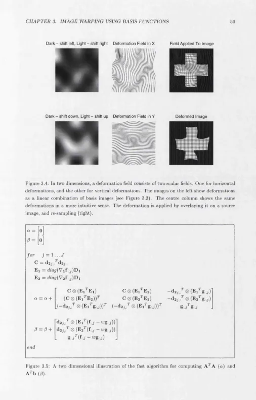
3.4 Deformation fields consist of a linear com bination of basis functions... 50
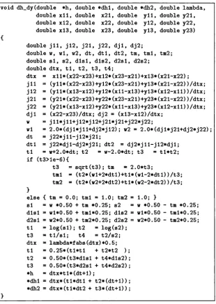
3.5 The fast algorithm ... 50
3.6 Exam ple tem plate im ages... 55
3.7 Two dimensional histogram s of tem plate im ages... 55
3.8 Sim ulated images of T l, T2 and PD weighted images... 56
3.9 Average for the images plotted against iteration num ber... 59
3.10 Number of iterations in which convergence to w ithin 1% is reached... 59
3.11 Param eter estim ates from reduced d a ta versus those from com plete d a ta ...60
3.12 Means and standard deviations of spatially normalised im ages... 61
3.13 Illustration of the effect of régularisation... 63
4.1 Triangular mesh used for 2D registration... 69
4.2 Probability density functions... 71
4.3 Tetrahedral mesh used for 3D registration... 72
4.4 A comparison of the different cost functions... 74
4.5 The six triangles whos Jacobian m atrices are influenced by the central point. . . . 75
4.6 C code for com puting the rate of change of the prior p o ten tial... 76
4.7 An illustration of how voxels are located within a tetrah ed ro n ...77
4.8 D em onstration using sim ulated d a ta ... 79
4.9 Dem onstration of the reversibility of the deform ations... 80
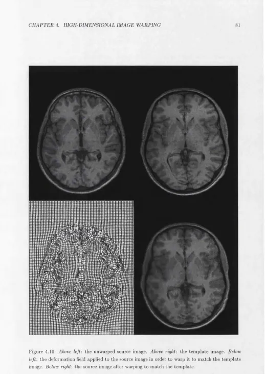
4.10 Example of 2D registration of brain images... 81
L IS T OF F IG U R E S 7
4.12 Deform ation fields from 3D registration... 83
4.13 Sym m etry of 3D deform ation fields... 84
4.14 Mean and standard deviation im ages...85
4.15 Affine registered im ages... 86
4.16 Bajsis function registered im ages... 87
4.17 High-dimensionally registered im ages...88
4.18 Rendered brain surfaces showing equivalent locations...89
4.19 M appings obtained by combining warps... 90
4.20 A comparison of a sym m etric with an asym m etric likelihood p o ten tial... 94
4.21 R otation and translations of a region, keeping surrounding points stationary. . . . 95
4.22 A shear has singular values not equal to one... 95
5.1 Prior probability im ages... 99
5.2 The segm entation m odel...100
5.3 A fiow diagram for the tissue classification...102
5.4 A lgorithm for com puting A k ^A k and A k ^ b k in two dim ensions... 105
5.5 Random ly generated m odulation fields... 106
5.6 Exam ple segm entation of real d a ta ...107
5.7 Classification of the sim ulated B rain Web im age... 108
5.8 Recovery of m odulation field... I l l 5.9 Segm entation accuracy w ith respect to m isregistration...112
5.10 Effects of partial volume on the intensity histogram s...113
5.11 Exam ple of autom atically cleaned up segmented im ages...115
6.1 Canonical correlation analysis using simulated d a ta ... 120
6.2 H istogram of correlation coefficients...124
6.3 Histogram s of t-scores from random ly generated tests... 126
6.4 Frequency of false positives...127
6.5 Tem plate and weighting im ages...129
6 .6 Means of spatially normalised images for each group... 129
6.7 Separation of subjects using canonical correlation analysis...132
6 .8 C aricatured shape differences... 133
6.9 Average shape differences... 134
6.10 W arping of same subject brain during Alzheimers disease progression...136
6.11 Volume changes during progression of Alzheimers disease...137
6.12 Polar decom position... 137
6.13 Mean of 58 warped hippocam pus im ages... 139
6.14 Random ly chosen warped images of hippocam pi... 140
6.15 Jacobian determ inant fields... 142
6.16 Histogram of correlation coefficients...143
6.17 Histograms of t-scores from random ly generated tests... 143
L IS T OF FIG U R E S 8
List o f Tables
C hapter 1
In trod u ction
C ontents
1.1 M otivation and A i m s ...10
1.1.1 Functional I m a g in g ... 10
1.1.2 C om putational N euroanatom y ... 12
1.2 O verview o f C h a p t e r s ...14
1.1
M otivation and A im s
The initial m otivation for this work was to develop improved m ethods of image registration for functional imaging. Much of it has now been incorporated into the S P M 99 package, and is used by several hundred researchers around the world for analysing functional im aging data. The second m otivation was to facilitate the development of m ethods for studying brain shape among different populations. Recently, the term computational neuroanatomy has been coined for this area of research. These areas are now reviewed in more detail.
1.1.1
Functional Im aging
The principle behind detecting activations using functional im aging m ethods such as Positron Em ission Tomography (PET) or functional Magnetic Resonance Imaging (fMRI) is essentially a voxel by voxel t-test on a series of images acquired under different conditions (Friston et a i,
1995d; Worsley & Friston, 1995). This analysis results in a statistical param etric m ap (SPM) showing significant differences in cerebral blood flow th a t are explained according to the different conditions experienced by the subject (or subjects) in the scanner.
The first m odalities used for this type of study were P E T and S P E C T {Single Photon Em ission Computed Tomography). Recent advances in MR m ethods, the large num ber of existing scanners, coupled with the relatively high cost of producing radioactive tracers, and the invasive nature of P E T and SPEC T have m eant th a t m ost studies currently use fMRI.
P E T and S PE C T m ethods involve generating images from the photons of radiation em itted by tracers injected into, or inhaled by, the subjects. Tracers used in P E T studies em it positrons
C H A P T E R 1. IN T R O D U C T IO N 11
when they decay, and include and ^®F, although m ost studies are based on identifying regional differences in cerebral blood flow, and involve injecting the subject with labelled water, or the subject breathing ^^0 labelled carbon dioxide. W hen a positron m eets an electron, the two annihilate each other resulting in the emission of two gam m a ray photons in opposite directions. By recording the paths of the gam m a ray pairs, it is possible to reconstruct a three dim ensional image of the tracer concentration. For P E T studies, a typical protocol m ay involve about 12 scans, with an injection of labelled water prior to each of them . The subject may have one task to do for six of the scans, and a different task for the other six. More active brain regions have a higher rate of blood flow, and so receive the tracer earlier th an the other areas. By imaging the brain as the radioactivity is entering, and com paring the images resulting from the different tasks, it is possible to create a picture of where the tasks have m ost influence over the cerebral blood flow.
The mechanisms of MRI are very different from those of P E T , and rely on the nuclei of certain atom s (normally ^H) absorbing and then re-em itting radio waves when in a m agnetic field. The frequency of the absorbed and em itted waves depends on the strength of the m agnetic field, so by varying the field over the head it is possible to record waves of different frequencies from different regions. Fourier transform m ethods are used to reconstruct images of where the signals em anate from. Depending on the properties of the surrounding tissue, the am plitudes of the signals will decay at different rates, so not only does MRI produce a m ap of the density of atom s, bu t it also says som ething about the environment in which the atom s are found.
Currently, the index of neuronal activity most commonly used for fMRI is the Blood Oxy genation Level Dependent (BOLD) contrast (Ogawa et a i, 1990). The assum ption is th a t an increase in neuronal activity within a brain region results in an increase in local blood flow, lead ing to reduced concentrations of deoxyhæmoglobin in the blood vessels. Unlike oxyhæ m oglobin, deoxyhæmoglobin has a differential m agnetic susceptibility in relation to the surrounding tissue. Therefore, relative decreases in deoxyhæmoglobin concentration lead to a reduction in local field inhom ogeneity and a slower decay of the MR signal, resulting in higher intensities in the images. fM RI allows whole brain images to be collected in about six seconds, giving it a much better tem poral resolution th an P E T (as there is typically a wait of about 10 m inutes between scans in order for the radiation from the previous scan to decay). T his m eans th a t hundreds of fMRI volumes are often collected for each subject.
C H A P T E R 1. IN T R O D U C T IO N 12
Motion correction is especially im portant for experim ents where subjects m ay move in the scanner in a way th a t is correlated with the different conditions (H ajnal et al., 1994). Even tiny system atic differences can result in a significant signal accum ulating over numerous scans. W ith out suitable corrections, artifacts arising from subject m ovement correlated w ith the experim ental paradigm m ay appear as activations. A second reason why m otion correction is im p o rtan t is th a t it increases sensitivity. The t-test is based on the signal change relative to the residual variance. T he residual variance is com puted from the sum of squared differences between the d a ta and the linear model to which it is fitted. Movement artifacts add to this residual variance, and so reduce the sensitivity of the test to true activations.
For studies of a single subject, sites of activation can be accurately localised by superim pos ing them on a high resolution structural image of the subject (typically a T l weighted MRI). T his requires registration of the functional images with the structural image. As in the case of m ovem ent correction, this is normally performed by optim ising a set of param eters describing a rigid body transform ation, but the m atching criterion needs to be more complex because the stru ctu ral and functional images normally look very different. A further use for this registration is th a t a more precise spatial norm alisation can be achieved by com puting it from a more detailed stru ctu ral image. If the functional and structural images are in register, then a warp com puted from the structural image can be applied to the functional images.
Sometimes it is desirable to warp images from a num ber of individuals into roughly the same stan d ard space to allow signal averaging across subjects. T his procedure is known as spatial norm alisation. Because different people m ay have different strategies for performing tasks in the scanner, spatial norm alisation of the images is useful for determ ining w hat happens generically over individuals. A further advantage of using spatially norm alised images is th a t activation sites can be reported according to their Euclidian co-ordinates w ithin a standard space (Fox, 1995). T he m ost comm only adopted co-ordinate system within the brain im aging com m unity is th a t described by Talairach &; Tournoux (1988), although new standards are now emerging th a t are based on digital atlases (Evans et a i, 1993; Evans et al., 1994; M azziotta et al., 1995).
1.1.2
C om p u tation al N eu roan atom y
A large num ber of approaches for characterising differences in the shape and neuroanatom ical configuration of different brains have recently emerged due to improved resolution of anatom ical hum an brain scans and the development of new sophisticated im age processing techniques.
One of the sim plest morphom etric approaches involves identifying shape changes w ithin single subjects by subtracting coregistered images acquired at different times. The changes could be because of a num ber of different reasons, but most are related to pathology. Because the scans are of the same subject, the first step for this kind of analysis involves registering the images together by a rigid body transform ation.
C H A P T E R 1. IN T R O D U C TIO N 13
, ^ % / / / / / / / ' . / / / / 1 . / / / .
y y I
-x-X'y'y’xyy% / / / / f / xnvvvNVVVVWVSSVNVVV swvSVWVN.
% \ \ I I / / * r > \ \ M I • r I I 1 I ^ < I I r I I I I ^ V I M r I / / M I I I <
iH iliir:';
t I I J I I I ' * ' I I I I I I t « * * M M I I I M I t I t I I 1 k I I I « « 1 1 I k k k I k I t « I k k k k k k k k » i
o o o o o o o o o o o o o o o o o o O o o o O O o o o o o o o o o o o o o o o O O O O O O O O O O O o0 0 0 O 0 O O 0 0 0 O 0 0 Oç q q q q q q0 0 ® 0 0 0 0 0 0 0 0 0 0 0 0 O o o o o O O O O O O e O O O O O O O O O O O O O o O n n O O O O O O o O O O O O o O O O O O O O O O O O O O O O O OO 00 0 o o o o o o O o o o S i o O O O O O O O O O O O O O O O O O O O O O O O O O O O 000 O O O O O ® ® ® ® ® « • « • • • O O O O O O O O O D O o O O O o o o o o ®
a O i i o «i O O o o » “ ° ?gooo»<>o ooo o o o o o » » o o o o o o o o
■■■■I
F ig u re 1.1: T h e te rm “d e fo rm a tio n -b a se d m o rp h o m e try ” will b e used to d escrib e m e th o d s o f s tu d y in g th e p o sitio n s o f s tru c tu re s w ith in th e b ra in (left), w h erea s th e te rm “te n so r-b a se d m o r p h o m e tr y ” will be used for m e th o d s th a t look a t local s h a p e s (rig h t). C u rre n tly , th e m a in a p p lic a tio n o f te n so r-b a se d m o rp h o m e try involves u sin g th e J a c o b ia n d e te r m in a n ts to e x a m in e th e re la tiv e v o lu m e s o f differen t stru c tu re s . H ow ever, th e re a re o th e r fe a tu re s o f th e J a c o b ia n m a tr ic e s t h a t co u ld be used, such as th o se re p re se n tin g e lo n g a tio n a n d c o n tra c tio n in d iffe ren t d ire c tio n s . T h e arro w s in th e p an e l on th e left show a b s o lu te d is p la c e m e n ts a fte r m a k in g a g lo b a l c o rre c tio n for r o ta tio n s a n d tr a n s la tio n s , w h ereas th e ellipses on th e rig h t show how th e sa m e circles w ould be d is to rte d in differen t p a r ts o f th e b ra in .
f u rth e r c h a ra c te ris e d u sing a n u m b e r of s ta tis tic a l p ro ce d u re s.
T h e te rm s d e fo rm a tio n -b a s e d a n d te n so r-b a se d m o rp h o m e try w ill b e used to d e n o te m e th o d s o f s tu d y in g b ra in sh a p e t h a t are b ased on d e fo rm a tio n fields. W h e n c o m p a rin g g ro u p s,
d e fo rm a tio n -b a s e d m o rp h o m e try (D B M ) uses d e fo rm a tio n fields to id e n tify differences in th e rel a tiv e p o sitio n s o f s tru c tu re s w ith in s u b je c ts ’ b ra in s. T e n so r-b a se d m o r p h o m e try (T B M ) refers to th o se m e th o d s t h a t id e n tify differences in th e local sh a p e o f b r a in s tr u c tu re s (see F ig u re 1.1).
C h a ra c te r is a tio n u sing D B M ca n be g lo b a l, p e r ta in in g to th e e n tire field as a single o b se r
v a tio n , o r ca n p ro ce ed on a voxel by voxel b asis to m a k e inferen ces a b o u t re g io n a lly specific p o s itio n a l differences. T h is sim p le ap p ro a c h to th e an a ly sis o f d e fo r m a tio n fields involves t r e a t in g th e m as v ec to r fields re p re se n tin g a b s o lu te d isp la c e m e n ts. H ow ever in th is fo rm , in a d d itio n to sh a p e in fo rm a tio n , th e v ecto r fields also c o n ta in in fo rm a tio n on p o s itio n a n d size t h a t is likely to co n fo u n d an a n a ly sis. M uch o f th e co n fo u n d in g in fo rm a tio n is first rem o v e d by g lo b a l r o ta tio n s ,
tr a n s la tio n s a n d a zo o m o f th e fields (B o o k ste in , 1997a).
D B M can be a p p lie d on a g lo b al scale to sim p ly id e n tify w h e th e r th e re are sig n ific an t d iffer ences in o verall s h a p e s (b ase d on a sm a ll n u m b e r o f p a ra m e te rs ) a m o n g th e b ra in s o f d iffe ren t
C H A P T E R 1. IN T R O D U C T IO N 14
statistic can be used for such simple comparisons between two groups of subjects (Bookstein, 1997a; Bookstein, 1999), bu t for more complex experim ental designs, a m ulti-variate analysis of covariance can be used to identify differences via the W ilk’s A statistic.
An alternative approach to DBM involves producing a statistical param etric m ap th a t locates any regions of significant positional differences among th e groups of subjects. An example of this approach involves using a voxel-wise Hotelling’s test on the vector field describing the displacements a t each and every voxel (Thompson & Toga, 1999; Gaser et al., 1999). The significance of any observed differences can be assessed by modelling the statistic field as a T^ random field (Cao & Worsley, 1999). Note th a t this approach does not directly localise brain regions w ith different shapes, but rather identifies those brain structures th a t are in relatively different positions.
If the objective is to localise structures whos shapes differ among groups, then some form of tensor-based m orphom etry is required to produce statistical param etric m aps of regional shape differences. A deform ation field th a t m aps one image to another can be considered as a discrete vector field. By taking the gradients at each element of the field, a Jacobian m atrix field is obtained, in which each element is a tensor describing the relative positions of neighbouring elements. M orphom etric measures derived from such a tensor field can be used to locate regions w ith different shapes. The field obtained by taking the determ inants at each point gives a m ap of structural volumes relative to those of a reference image (Freeborough & Fox, 1998; Gee & Bajcsy, 1999). Statistical param etric m aps of these determ inant fields can then be used to compare the anatom y of groups of subjects. A number of other measures derived from tensor fields have been used by other researchers, and these are described by Thom pson and Toga (1999).
A nother form of m orphom etry involves examining the local com position of brain images. Grey and white m a tte r voxels can be identified by image segm entation, before applying m orphom etric m ethods to study the spatial distribution of the tissue classes. These techniques will be referred to as voxel-based m orphom etry (VBM). Currently, the difficulty of com puting very high resolution deform ation fields (required for TBM at small scales) makes voxel-based m orphom etry a simple and pragm atic approach to addressing small scale differences th a t is within the capabilities of m ost research units.
To sum m arise, com putational neuroanatom ic techniques can either use the deform ation fields themselves or use these fields to normalise images th a t are then entered into an analysis of regionally specific differences. In this way, inform ation about overall shape (deformations fields) and residual anatom ic differences inherent in the d a ta (registered images) can be partitioned.
1.2
O verview o f Chapters
T he rem aining chapters of this thesis are organised as follows.
R ig id B o d y R eg istra tio n
C H A P T E R 1. IN T R O D U C T IO N 15
w ith head movement, so rigid body transform ations can be used to model different head positions of the same subject. R egistration m ethods described in this chapter include within m odality, or between different m odalities such as P E T and MRI. M atching of two images is perform ed by finding the rotations and translations th a t optimise some m utual function of the images. W ithin m odality registration generally involves m atching the images by minimising the sum of squared difference between them . For between m odality registration, the m atching criterion needs to be more complex. A m ethod for co-registering brain images of the same subject th a t have been acquired in different m odalities is presented. The basic idea is th a t instead of m atching two images directly, one performs interm ediate within m odality registrations to two tem plate images th a t are already in register. One can use a least squares m inim isation to determ ine the affine transform ations th a t m ap between the tem plates and the images. By incorporating suitable constraints, a rigid body transform ation th a t directly m aps between the images can be extracted from these more general affine transform ations. A further refinement capitalises on the im plicit norm alisation of both images into a standard space. T his facilitates partitioning both original images into homologous tissue classes. Once extracted, the p artitions are jointly m atched further increasing the accuracy of the co-registration.
Im age W arping w ith B asis Functions
This chapter describes the steps involved in registering images of different subjects into roughly the same co-ordinate system, where the co-ordinate system is defined by a tem plate image (or series of images). The m ethod only uses up to a few hundred param eters, so can only model global brain shape. It works by estim ating the optim um coefficients for a set of bases, by minimising the sum of squared differences between the tem plate and source image, while sim ultaneously m aximising the smoothness of the transform ation using a m axim um a posteriori (MAP) approach. In order to adopt the MAP approach, it is necessary to have estim ates of the likelihood of obtaining the fit given the data, which requires prior knowledge of spatial variability, and also knowledge of the variance associated with each observation. True Bayesian approaches assume th a t the variance associated w ith each voxel is already known, whereas the approach developed here is a type of Em pirical Bayesian m ethod, which attem pts to estim ate this variance from the residual errors. Because the registration is based on sm ooth images, correlations between neighbouring voxels are considered when estim ating the variance. This makes the same approach suitable for the spatial norm alisation of both high quality M R images, and low resolution noisy P E T images. A fast algorithm has been developed th a t utilises Taylor’s Theorem and the separable nature of the basis functions, meaning th a t m ost of the nonlinear spatial variability between images can be autom atically corrected within a few minutes.
C H A P T E R 1. IN T R O D U C T IO N 16
m em brane energy.
H igh D im en sion al Im age W arping
T his chapter is also about warping brain images of different subjects to the same stereotactic space. However, unlike C hapter 3, this m ethod uses thousands or millions of param eters, so is potentially able to obtain much more precision. A high dim ensional m odel is used, whereby a finite element approach is employed to estim ate translations a t the location of each voxel in the tem plate image. Bayesian statistics are used to obtain a m axim um a posteriori (MAP) estim ate of the deform ation field. The validity of any registration m ethod is largely based upon the prior knowledge about the variability of the estim ated param eters. In this approach it is assumed th a t the priors should have some form of symmetry, in th a t priors describing the probability distribution of the deformations should be identical to those for the inverses (i.e., warping brain A to brain B should not be different probablistically from warping B to A). The fundam ental assum ption is th a t the probability of stretching a voxel by a factor of n is considered to be the sam e as the probability of shrinking n voxels by a factor of n~^. The penalty function of choice is based upon the singular values of the Jacobian m atrices having log-normal distributions, which enforces a continuous one-to-one mapping. A gradient descent algorithm is presented th a t incorporates the above priors in order to obtain a MAP estim ate of the deformations. Further consistency is achieved by registering images to their “averages” , where this average is one of both intensity and shape.
S eg m en ta tio n
A tissue classification m ethod was originally developed to be p a rt of the between m odality regis tratio n procedure described in C hapter 2, bu t the classification results are also useful for various types of m orphom etry, as well as having potential applications in other registration techniques. T his chapter describes a m ethod of segmenting MR images into different tissue classes, using a modified Gaussian M ixture Model. By knowing the prior spatial probability of each voxel being grey m atter, white m atter or cerebro-spinal fluid, it is possible to obtain a more robust classifica tion. In addition, a step for correcting intensity non-uniform ity is also included, which makes the m ethod more applicable to images corrupted by sm ooth intensity variations. Evaluations of the m ethod show th a t the non-uniformity correction improves the segm entation of images containing this artifact.
M o rp h o m etry
T he chapter on m orphom etry covers three principle m orphom etric m ethods, th a t will be called
voxel-based, deformation-based and tensor-based m orphom etry.
C H A P T E R 1. IN T R O D U C T IO N 17
statistical tests are performed which compare the sm oothed grey-m atter images from the groups. Corrections for m ultiple com parisons are m ade using the theory of G aussian random fields. This chapter describes the steps involved in VBM, and provides evaluations of the assum ptions m ade about the statistical distribution of the data.
Deform ation-based m orphom etry (DBM) is a m ethod for identifying macroscopic anatom ical differences am ong the brains of different populations of subjects. The m ethod involves spatially norm alising the structural M R images of a num ber of subjects so th a t they all conform to the sam e stereotactic space. M ultivariate statistics are then applied to the param eters describing the estim ated nonlinear deform ations th a t ensue. To illustrate the m ethod, the gross m orphom etry of m ale and female subjects are compared. Brain asym metry, the effect of handedness, and the interactions among these effects are also assessed.
C hapter 2
R igid B o d y R egistration
C on ten ts
2.1 I n t r o d u c t i o n ... 18
2.2 A fhne T r a n s fo r m a tio n s ... 19
2.2.1 P aram eterising a Rigid Body T rc in s fo rm a tio n ... 21
2.2.2 Working w ith Volumes of Differing or A nisotropic Voxel Sizes . . . . 22
2.2.3 Left- and R ight-handed C o-ordinate S y s t e m s ... 22
2.3 R esam p lin g I m a g e s ...23
2.4 O p t i m i s a t i o n ... 26
2.5 W ith in M o d ality Im age R egistration ...27
2.5.1 M e th o d s ... 28
2.5.2 Residucil A rtifacts from P E T and f M R I ... 30
2.6 B etw een M o d ality Im age R egistration ...31
2.6.1 M e th o d s ... 32
2.6.2 E valuation ... 35
2.1
Introduction
Rigid body registration is normally used for registering images of the same subject. This chapter describes m ethods of within subject registration for images of the same or different m odalities.
For every image registration, the spatial transform ation should be described by a set of pa ram eters. In three dimensions, rigid registration requires six param eters: three translations and three rotations. There are two steps involved in registering a pair of images together. There is the
registration itself, whereby the param eters describing a transform ation are estim ated. Then there is the transformation, where one of the images is transform ed according to the set of param eters.
A t its simplest, image registration involves estim ating a m apping between a pair of images. One im age is assumed to remain stationary (the target or tem plate image), whereas the other (the source image) is spatially transform ed to m atch it. In order to transform the source to m atch the target, it is necessary to determ ine a m apping from each voxel position (x) in the target to a corresponding position (y) in the source. The source is then resampled at the new positions. The
C H A P T E R 2. R IG ID B O D Y R E G IS T R A T IO N 19
vector function y can be thought of as a function of x, and a set of transform ation param eters q th a t are estim ated in order to register the images.
This chapter will touch first on how rigid transform ations are param eterised in term s of affine transform ations. The next section explains how the images are transform ed via the process of resam pling, before the optim isation section explains how the best values for the param eters (q) are estim ated. The simplest form of within subject registration involves registering together two images of the same modality. A m ethod for doing this is briefly described, before the final section describes a more complex technique for performing between m odality registration.
2.2
Affine Transform ations
Rigid body transform ations are a subset of the more general affine transform ations. For each point (x i, X2, X3) in an image, an affine m apping can be defined into the co-ordinates of another
space (y i,y2,2/3)- This is expressed as:
y i = 77111x1 - f m i 2X2 + 77113X3 + 77114
V2 = 77121X1 - f 77122^2 + 77123373 + 77124 (2.1) ys = 77131X1 - f 77132 X 2 + 77133X3 + 77134
T his m apping is often expressed as a simple m atrix m ultiplication (y = M x ) :
7/1 7/2 ys
1
m il m i2 mi3 mi4 mgi m22 m23 ^ 2 4 m3i m32 77133 77134
0 0 0 1
X i
X 2 X 3
1
(2.2)
T he elegance of form ulating these transform ations in term s of m atrices is th a t several trans form ations can be combined simply by multiplying the m atrices together to form a single m atrix. T his m eans th a t repeated resampling of d a ta can be avoided when reorienting an image.
T r a n s la tio n s
T ranslations are simple to im plem ent. If a point x is to be translated by q units, then the transform ation is simply:
y = x + q
In m atrix term s, this transform ation can be considered as:
7/1 1 0 0 gi Xi
yz 0 1 0 Ç2 X2
ys 0 0 1 Ç3 X3
1 0 0 0 1 1
(2.3)
(2.4)
R o t a t io n s
C H A P T E R 2. R IG ID B O D Y R E G IS T R A T IO N 20
radians around the origin, can be generated by the transform ation:
yi = cos{9)xi + sin {6) x2
U2 = - s i n {0)x i + cos{9) x2
(2.5)
This is another example of an affine transform ation. For the three dim ensional case, there are three orthogonal planes th a t an object can be rotated in. For simplicity, the planes of rotation are norm ally expressed as being around the axes. A rotation of q\ radians about the first (x) axis is norm ally called pitch, and is performed by:
(2.6)
Similarly, rotations about the second (y) and third {z) axes (called roll and yaw respectively) are carried out by the following matrices:
2/1 ’l 0 0 o' X i
2/2 0 cos(9i) sm (9i) 0 X2
2/3 0 —sin{qi) cos{qi) 0 X3
1 0 0 0 1 1
cos{q2) 0 sin{q2) o' cog(93) sin (93) 0 o'
0 1 0 0
and -sin iq a ) cos(93) 0 0
- s in { q2) 0 cos(92) 0 0 0 1 0
0 0 0 1 0 0 0 1
R otations are combined by m ultiplying these m atrices together in the appropriate order. The order in which the operations are perform ed is im portant. For example, a rotation about the first axis of 7t/ 2 radians followed by an equivalent rotation about the second axis would produce a very different result to th a t obtained if the order of the operations was reversed.
Z oom s
T he affine transform ations described so far will perform purely rigid m appings. Zooms are needed to change the size of an image, or to work w ith images whos voxel sizes are not isotropic, or differ between images. These merely represent scalings along the orthogonal axes, and can be represented via:
2/1 2/2 2/3 1
gi 0 0 0
0 92 0 0
0 0 93 0
0 0 0 1
Xi
1
(2.T)
C H A P T E R 2. R IG ID B O D Y R E G IS T R A T IO N 21
S h e a r s
Shearing by param eters q\ , Q2 and 93 can be performed by the following m atrix:
1 0 0 ?2 93 1 0
A shear by itself is not a rigid body transform ation, bu t it is possible to combine shears in order to generate rigid rotations. For a simple two dimensional case, a m atrix encoding a rotation of 9 radians about the origin (see Section 2.5) can be constructed by m ultiplying together three m atrices th a t effect shears;
(2.8)
T his approach has been useful for rigid registration of M R images (Eddy et a i, 1996), and subsequently improved by a more efficient reform ulation for three dim ensional transform ations (Cox & Jesmanowicz, 1999).
cos{9) sin{$) o' '1 tan{9/2) o' 1 0 o' '1 tan{9/2) o'
—sin {6) cos{9) 0 = 0 1 0 sin{9) 1 0 0 1 0
0 0 1 _0 0 1 0 0 1 0 0 1
2.2.1
P aram eterisin g a R igid B o d y T ransform ation
W hen registering a pair of images together via a rigid body transform ation, it is necessary to estim ate six param eters th a t describe the rigid-body transform ation m atrix. There are m any ways of param eterising a rigid body transform ation in term s of six param eters (q), b u t the param eterisation chosen here is:
M = T R where:
T =
91 92 93
1
(2.9)
( 2 . 10)
and:
R =
1 0 0 o' 005(95) 0 sin (95) o' 0 0 5(95) 5in(96) 0 o'
0 00 5(94) sin{q4) 0 0 1 0 0 - s i n (96) 0 0 5(95) 0 0
0 - s i n (9 4) 005(94) 0 -sin {q ^) 0 005(95) 0 0 0 1 0
0 0 0 1 0 0 0 1 0 0 0 1
(2.11)
E xtracting the param eters q from M is relatively straightforw ard. D eterm ining the tran sla tions is trivial, as they are simply contained in the fourth colum n of M . This ju st leaves the rotations:
R =
C5C6 cgSg S5 0
—S4S5C6 — C4S6 —S4S5S6 4" C4C6 S4C5 0 —C4S5C6 + S4SQ —C4S5S6 ~ &4C6 C4C5 0
0 0 0 1
C H A P T E R 2. R IG ID B O D Y R E G IS T R A T IO N 22
where 5 4, S5 and sg are the sines, and C4, C5 and cq are the cosines of param eters 94, and gg respectively. Therefore, providing th a t cg is not zero, then:
9 5 = s m “ ^ (ri3)
94 = atan2{r23/005(95), rz3/cos{q^)
96 = afan 2 (ri2 /co s(g 5 ),rii/co s(9 5 ) (2.13) where atan2 is the four quadrant inverse tangent. See Section 6.4 for m ore on decomposing afhne transform ations containing zooms and shears.
2.2.2
W orking w ith V olum es o f D iffering or A n iso tro p ic V oxel Sizes
Im age voxel sizes need be considered when performing rigid body registration. Often, the images (say
f
and g) will have voxels th a t are anisotropic. The dimensions of the voxels are also likely to differ between images of different modalities. For simplicity, a Euclidean space is used, where m easures of distance are expressed in millimetres. R ather th a n interpolating the images such th a t the voxels are cubic and have the same dimensions in all images, one can simply define affine transform ation m atrices th a t m ap from voxel co-ordinates into this Euclidean space. For example, if imagef
is of size 128 x 128 x 43 and has voxels th a t are 2.1mm x 2.1mm x 2.45mm, the following m atrix can be defined:M f =
2.1 0 0 -1 3 4 .4 0 2.1 0 -1 3 4 .4
0 0 2.45 -52.675
0 0 0 1
(2.14)
This transform ation m atrix m aps voxel co-ordinates to a Euclidean space who’s axes are parallel to those of the image and distances are measured in millimetres, with the origin at the centre of the image. A sim ilar m atrix can be defined for g (M g). Because m odern MR image form ats such as SPI (S tandard P roduct Interconnect) generally contain inform ation about image orientations in their headers, it is possible to extract this inform ation to autom atically com pute values for M f
or M g. This makes it possible to easily register images together th a t were originally acquired in com pletely different orientations.
T he objective of any co-registration is to determ ine the rigid body transform ation th a t m aps the co-ordinates of image g, to th a t of f . To accomplish this, a rigid body transform ation m atrix M r is determ ined, such th a t M f ~^M r~^M g will m ap from voxels in g to those in f . The inverse of this m atrix m aps from
f
to g. Once M r has been determ ined, M f can be set to M r M f . From there onwards the m apping between the voxels of the two images can be achieved by M f~ ^M g . Similarly, if another image(h)
is also co-registered to image g in the same m anner, then not only is there a m apping fromh
and g (via M g “ ^M h), but there is also one fromh
tof
which is sim ply M f “ ^M h (derived from M f “ ^M gM g“ ^M h).2 .2 .3
Left- and R ight-handed C o-ordinate S y stem s
C H A P T E R 2. RIG ID B O D Y R E G IST R A T IO N 23
Left-Handed
Right-Handed
1
0.5
0
1
0.5 0.5
0 0
z
1
0.5
0.
0
0.5 0.5
1 0
z
Figure 2.1: Left- and right-handed co-ordinate systems.
(often referred to as the x direction) increases from left to right, the second dimension goes from posterior to anterior (back to front) and the third dimension increases from inferior to superior (bottom to top). The axes can be rotated by any angle, and they still retain their handedness. An affine transform ation th at m aps between left and right-handed co-ordinate systems has a negative determ inant, whereas one th a t maps between co-ordinate systems of the same kind will have a positive determ inant. Because the left and right sides of a brain have similar appearances, care m ust be taken when reorienting brain image volumes. Consistency of the co-ordinate systems can be achieved by performing any reorientations using affine transform ations, and checking the determ inants of the transform ation matrices.
2.3
Resam pling Images
Once there is a mapping between the original and transformed co-ordinates of an image, it is necessary to resample the image in order to apply the spatial transform . Spatially transforming images is usually implemented as a “pulling” operation (where pixel values are pulled from the original image into their new location) rather than a “pushing” one (where the pixels in the original image are pushed into their new location). This involves determ ining for each voxel in the transformed image, the corresponding intensity in the original image. Usually, this requires sampling between the centres of voxels, so some form of interpolation is needed.
The simplest approach is to take the value of the closest neighbouring voxel. This is referred to as nearest neighbour or zero-order hold resampling. This has the advantage th a t the original voxel intensities are preserved, but the resulting image is degraded quite considerably.
Another approach is to use tri-linear interpolation {first-order hold) to resample the data. This is slightly slower than nearest neighbour, but the resulting images have a less “blocky” appearance. However, tri-linear interpolation has the effect of losing some high frequency inform ation from the image.
C H A P T E R 2. R IG ID B O D Y R E G IS T R A T IO N 24
(a) (b) [q] (c) (d)
(e) (f) [r] (g) (h)
{u)
(i) Û) [s] (k) (1)
(m) (n) [t] (0) (P)
Figure 2.2: Illustration of image interpolation in two dimensions. Points a through to p represent the original regular grid of pixels. Point u is the point who’s value is to be determ ined. Points q
to t are used as interm ediates in the com putation.
th a t there is a regular grid of pixels at co-ordinates Xa,ya to Xp,pp, having intensities Va to Vp,
and th a t the point to resample is at u. The value at points r and s are first determ ined (using linear interpolation) as follows:
{ X g - X r ) v f - f { X r ~ X f ) V g
Vr =
X g X f
_ { X k - X s ) v j - f (a;, - X j ) v k
— %
X k X j
Then is determ ined by interpolating between Vr and Vg : _ (Vu - y , ) V r + ( Vr - Vu)v,
V t - V )
(2.15)
(2.16)
T he extension of the approach to three dimensions is trivial.
R ath er th an using only the 8 nearest neighbours (in 3D) to estim ate the value at a point, more neighbours can be used in order to fit a sm ooth function through the points, and then read off the value of the function at the desired location. Polynomial interpolation is one such approach (zero- and first-order hold interpolations are simply low order polynom ial interpolations). It is now illustrated how Vq can be determ ined from pixels a to d. The coefficients (q) of a polynomial th a t runs through these points can be obtained by computing:
q =
1 0 0 0
- 1
Va
1 {Xb - X a ) { Xb - X a ) ^ (X6 - X a ) ^ Vb
1 [ Xc - X a ) { Xc - X a ) ^ { Xc - X a ) ^ Vc
1 { Xd - X a ) { X d - X a ) ^ { X d - Xa ) ^ _ y d _
C H A P T E R 2. RIG ID B O D Y R E G IS T R A T IO N 25
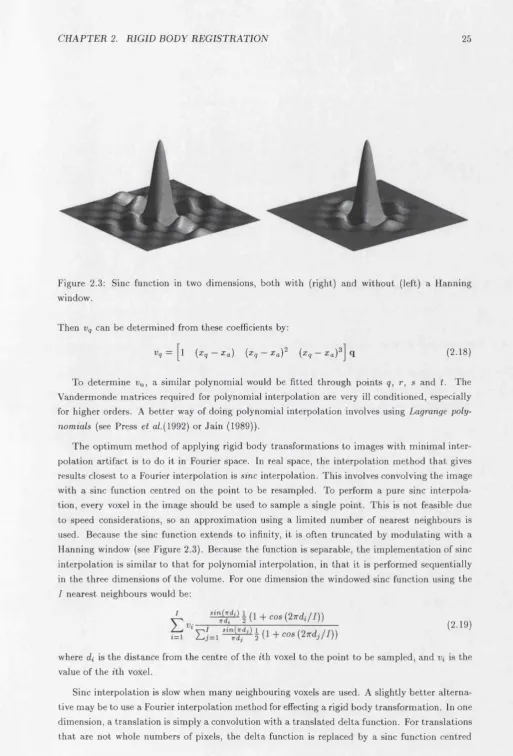
Figure 2.3: Sine function in two dimensions, both with (right) and without (left) a Hanning window.
Then Vq can be determ ined from these coefficients by:
v„ = 1 {^q ^a) i^q ^a) {Xq #a)' (2.18)
To determ ine v^, a similar polynomial would be fitted through points q, r, s and t. The Vandermonde m atrices required for polynomial interpolation are very ill conditioned, especially for higher orders. A better way of doing polynomial interpolation involves using Lagrange poly nomials (see Press et a/.(1992) or Jain (1989)).
The optim um m ethod of applying rigid body transform ations to images with m inim al inter polation artifact is to do it in Fourier space. In real space, the interpolation m ethod th at gives results closest to a Fourier interpolation is sine interpolation. This involves convolving the image with a sine function centred on the point to be resampled. To perform a pure sine interpola tion, every voxel in the image should be used to sample a single point. This is not feasible due to speed considerations, so an approxim ation using a limited num ber of nearest neighbours is used. Because the sine function extends to infinity, it is often truncated by m odulating with a Hanning window (see Figure 2.3). Because the function is separable, the im plem entation of sine interpolation is sim ilar to th at for polynomial interpolation, in th a t it is performed sequentially in the three dimensions of the volume. For one dimension the windowed sine function using the
I nearest neighbours would be:
(2.19)
where d,- is the distance from the centre of the zth voxel to the point to be sampled, and n, is the value of the zth voxel.
C H A P T E R 2. R IG ID B O D Y R E G IS T R A T IO N 26
a t the translation distance. The use of fast Fourier transform s m eans th a t the convolution can be perform ed most rapidly as a m ultiplication in Fourier space. It is clear how translations can be perform ed in this way, bu t rotations are less obvious. One way th a t rotations can be effected involves replacing the rotations by a series of shears as described previously (Section 2.2). A shear sim ply involves translating different rows or columns of an image by different am ounts, so each shear can be performed by a series of one dimensional convolutions in Fourier space. Alter natively, the m ethod of rotating and translating using shears can also be done using a windowed sine or polynom ial interpolation. Each interpolation is in ju st one dimension, requiring much less com putation than it would in three dimensions.
In addition to resampling images, m any image registration m ethods also require the image gradients to be com puted. This procedure is sim ilar to the straightforw ard interpolation m ethods described above.
2.4
O ptim isation
The objective of optim isation is to determ ine the values for a set of param eters for which some function of the param eters is minimised (or m axim ised). One of the sim plest cases involves deter m ining the optim um param eters for a model in order to m inimise the sum of squared differences between a model and a set of real world d a ta (%^). Norm ally there are m any param eters, and it is not possible to exhaustively search through the whole param eter space. The usual approach is to m ake an initial param eter estim ate, and begin iteratively searching from there. At each iteration, the m odel is evaluated using the current param eter estim ates, and com puted. A judgem ent is then m ade about how the param eter estim ates should be modified, before continuing on to the next iteration. The optim isation is term inated when some convergence criterion is achieved (usually when stops decreasing).
T he image registration approach described here is essentially an optim isation. One image (the source image) is spatially transform ed so th a t it m atches another (the target image), by m inim ising %^. The param eters th a t are optimised are those th a t describe the spatial tran s form ation (although there are often other nuisance param eters required by the model, such as intensity scaling param eters). For rigid registration, the algorithm chosen (Friston et a l, 1995c) is Gauss-Newton optim isation, and it is illustrated here;
Suppose th a t 6»(q) is the function describing the difference between the source and target images at voxel i, when the vector of model param eters have values q. For each voxel, a first approxim ation of Taylor’s Theorem can be used to estim ate the value th a t this difference will take if the param eters q are decreased by t:
dqi dq2
This allows the construction of a set of simultaneous equations (of the form A t the values th a t t should assume to in order to minimise 6i(q — t)^:
9fei(q)
d q i
db-jQl)
d q i
dbijq) dq2
Q<>2(q)
dq2
'h 6i(q )
^2(q)
(2.20) b ) for estim ating
C H A P T E R 2. RIG ID B O D Y R E G IS T R A T IO N 27
From this, an iterative scheme can be derived for improving the param eter estim ates. For iteration
n, the param eters q are updated as:
q(n + l) _ „(r»)= q(") - (A ^ A ) A ^ b (2.22)
where A =
9fci(q) 9fei(q)
dqi dq<2
963(g) 962(g)
dqi dq-2
6i(q) and b = &2(q)
This process is repeated until can no longer be decreased - or for a fixed num ber of iterations. T here is no guarantee th a t the best global solution will be reached, because the algorithm can get caught in a local minimum. To reduce this problem, the starting estim ates for q should be set as close as possible to the optim um solution. The num ber of potential local m inim a can also be decreased by working with sm ooth images. This also has the effect of m aking the first order Taylor approxim ation more accurate for larger displacements. Once the registration is close to the final solution, it can continue with less sm ooth images.
In practice, A ^ A and A ^ b from Eqn. 2.22 are often com puted ‘on the fly’ for each iter ation. By com puting these m atrices using only a few rows of A and b at a tim e, much less com puter memory is required than is necessary for storing the whole of m atrix A . Also, the p artial derivatives dhi{q)/dqj can be rapidly com puted from the gradients of the images using the chain rule.
It should be noted th a t element i of A ^ b is equal to and th a t element i , j of A ^ A is approxim ately equal to ^ Q^ Qg. (one half of the Hessian m atrix, often referred to as the curvature m atrix - see Press et a/.(1992). Section 15.5). Another way of thinking about the optim isation is th a t it fits a quadratic function to the error surface at each iteration. Successive param eter estim ates are chosen such th a t they are at the m inim um point of this quadratic (illustrated for a single param eter in Figure 2.4).
2.5
W ith in M odality Im age R egistration
W ithin m odality image registration has a number of uses, both w ithin m orphom etry and for processing functional images. M orphometric studies sometimes involve looking at changes in brain shape over tim e, often to study the progression of a disease such as Altzheimers, or to m onitor tu m o u r growth or shrinkage. Differences between structural MR scans acquired a t different times are identified, by first co-registering the images and then looking at the difference between the registered images. Rigid registration can also be used as a pre-processing step before using nonlinear registration m ethods for identifying shape changes (Freeborough & Fox, 1998).
C H A P T E R 2. RIG ID B O D Y R E G IS T R A T IO N 28
20
Starting estim ate
15 Iteration 1
I
1 10
Iteration 2 1
g 5
0
Minimum
0 20 40
D isplacem ent from true solution
60 80 100
Figure 2.4: The optimisation can be thought of as fitting a series of quadratics to the error surface. Each param eter update is such th a t it falls at the m inim um of the quadratic.
at the same time as the mean, in order to provide better weighting for the registration. Voxels with a lot of variance should be given lower weighting, whereas those with less variance should be weighted more highly.
2.5.1
M ethods
To register a source image
f
to a reference image g, a six param eter rigid body transform ation (param eterised by q\ to ge) would be used. To perform the registration, a num ber of points in the reference image (each denoted by x, ) are compared with points in the source im age (denoted by M x j, where M is the rigid body transform ation m atrix constructed from the six param eters). The images may be scaled differently, so an additional intensity scaling param eter (g?) may be included in the model. The param eters (q) are optimised by minimising the sum of squared differences^ between the images according to the algorithm described in Sections 2.2.1 and 2.4 (Eqn. 2.22). The function th at is minimised is:^ (/(M X i) - q j g M ) ' (2.23)
C H A P T E R 2. R IG ID B O D Y R E G IS T R A T IO N 29
where M = M f ^M r ^Mg, and M r is constructed from param eters q (refer to Section 2.2.2). Vector b is generated for each iteration as:
b =
/ ( M x i ) - 97^ (x i)
/(M x 2 ) - q7g{x2) (2.24)
Each column of m atrix A is constructed by differentiating b w ith respect to param eters qi to gy: a/(Mxi)
A =
d qi dq2 • • • dqe 3\ ^1)
df{Mx2) a/(Mxa) a/(Mx2) _ / \
agi dqaoo 2 • • • aoK y \ ^2) (2.25)
Because non-singular affine transform ations are easily invertible, it is possible to make the registration m ore robust by also considering what happens w ith the inverse transform ation. By swapping around the source and reference image, the registration problem also becomes one of minimising:
V i ) - 9 r V ( y j)) ' (2.26)
In theory, a more robust solution could be achieved by sim ultaneously including the inverse transform ation to make the registration problem sym m etric (Woods et a i, 1998a). The cost function would then be:
^ ( / ( M x i ) - q 7 9 { ^ i ) ) ^ 4 - ^ 2 ^ ( ^ ( M V j ) ~ 9? V ( y j ) ) ' (2.27) Normally, the intensity scaling of the image pair will be sim ilar, so equal values for the weighting factors (Ai and A2) can be used. M atrix A and vector b would then be form ulated as:
A f ( /( M x i) - 979(x i)) A f ( /( M x2) - 9 7 9(xz))
and
b =
A|(flf(M ^yi) - 9 7 V (y i))
M (9 (M -^ y 2 ) - 9 7 V ( y 2 ) )
A =
\ 2 d f ( M x i ) dqi
\ 2 ^1 dqi
\ h d g { M l y i ) agi \ 2 9g ( M V 2 ) ' ' 2 d q i
- A . b ( x . ) ■
a| m > ^ A J , f V ( y i )
A |“ i ^ A |, f V ( y 2 )
(2.28)
(2.29)
C H A P T E R 2. R IG ID B O D Y R E G IS T R A T IO N 30
2 .5 .2
R esid u al A rtifacts from P E T and fM R I
Even after realignm ent, there may still be some m otion related artifacts rem aining in functional d ata. After retrospective realignment of P E T images w ith large movements, the prim ary source of error is due to incorrect attenuation correction. In emission tom ography m ethods, m any photons are not detected because they are attenuated by the su b ject’s head. Normally, a transm ission scan (using a moving radioactive source external to the subject) is acquired before collecting the emission scans. The ratio of the num ber of detected photon pairs from the source, w ith and w ithout a head in the field of view, produces a m ap of the proportion of photons th a t are absorbed along any line-of-response. If a subject moves between the transm ission and emission scans, then the applied attenuation correction is incorrect because the emission scan is no longer aligned w ith the transm ission scan. There are methods for correcting these errors (Andersson et a/., 1995), b u t they are beyond the scope of this thesis.
In fMRI, there are m any sources of m otion related artifacts. T he m ost obvious ones are:
• Interpolation error from the resampling algorithm used to transform the images can be one of the m ain sources of m otion related artifacts. W hen the image series is resam pled, it is im p o rtan t to use a very accurate interpolation m ethod such as sine or Fourier interpolation. • W hen MR images are reconstructed, the final images are usually the m odulus of the initially
complex data, resulting in any voxels th a t should be negative being rendered positive. This has im plications when the images are resampled, because it leads to errors at the edge of the brain th a t can not be corrected however good the interpolation m ethod is. Possible ways to circumvent this problem are to work w ith complex d a ta , or possibly to apply a low pass filter to the complex d a ta before taking the modulus.
• T he sensitivity (slice selection) profile of each slice also plays a role in introducing artifacts (Noll et a i, 1997).
• fM RI images are spatially distorted, and the am ount of distortion depends p artly upon the position of the subject’s head within the m agnetic field. Relatively large subject m ovem ents result in the brain images changing shape, and these shape changes can not be corrected by a rigid body transform ation (Jezzard &: Clare, 1999).
• Each fMRI volume of a series is currently acquired a plane a t a tim e over a period of a few seconds. Subject movement between acquiring the first and last plane of any volume leads to another reason why the images may not strictly obey the rules of rigid body m otion. • A fter a slice is magnetised, the excited tissue takes tim e to recover to its original state, and
the am ount of recovery th a t has taken place will influence the intensity of the tissue in the image. O ut of plane movement will result in a slightly different p art of the brain being excited during each repeat. This means th a t the spin excitation will vary in a way th a t is related to head motion, and so leads to more movement related artifacts.
• G host artifacts in the images do not obey the same rigid body rules as the head, so a rigid ro tatio n to align the head will not m ean th a t the ghosts are aligned.