1573
Volume 66 158 Number 6, 2018
TEXT‑MINING IN STREAMS OF
TEXTUAL DATA USING TIME SERIES
APPLIED TO STOCK MARKET
Pavel Netolický
1, Jonáš Petrovský
1, František Dařena
11 Department of Informatics, Faculty of Business and Economics, Mendel University in Brno, Zemědělská 1, 613 00 Brno, Czech Republic
To cite this article: NETOLICKÝ PAVEL, PETROVSKÝ JONÁŠ, DAŘENA FRANTIŠEK. 2018. Text‑Mining in Streams of Textual Data Using Time Series Applied to Stock Market. Acta Universitatis Agriculturae et Silviculturae Mendelianae Brunensis, 66(6): 1573 – 1580.
To link to this article: https: / / doi.org / 10.11118 / actaun201866061573
Abstract
Each day, a lot of text data is generated. This data comes from various sources and may contain valuable information. In this article, we use text mining methods to discover if there is a connection between news articles and changes of the S & P 500 stock index. The index values and documents were divided into time windows according to the direction of the index value changes. We achieved a classification accuracy of 65 – 74 %.
Keywords: machine learning, text mining, stock market, data stream
INTRODUCTION
In recent years, big data have emerged as an important addition to traditional data sources derived from behavioral research (which generally involves data collection via either surveys or accessing administrative records, followed by analysis). The term “big data” is evolving and refers to extremely large data sets derived from the Internet, mobile devices, sensors, and other sources, as well as the wealth of available information that, if analyzed appropriately, can reveal valuable insights (Manyika, 2011).
Lot of current research has been focusing on incorporating the vast amount of data available online into models of various social and economic phenomena in miscellaneous areas. The data, which is generated not only by domain experts but also by regular people, can provide new perspectives and potentially complementary information to conventional quantitative and objective evidence.
A huge amount of data is constantly being generated by people and organizations. The data
often comes from nontraditional and contemporary information sources and environments, like social networks or microblogging sites.
The data has typically a form of unstructured texts that are published by different types of subjects, without the time and spatial limits. The speed of data creation is rapidly growing and we use the term “data stream” – a possibly unbounded sequence of data records – for the constant flow of new data (Aggarwal, 2007).
Data streams may be of various data types (text, image, numeric) and come from different application areas (computer networks monitoring, scientific experiments, internet search, social networks etc.). In comparison to batch processing (for which we have all data available at once), data streams processing provides a different approach, because it reflects the concept changing over time (Gama, 2010).
attractive application of data streams lies in examining data generated in the financial market. Kargupta et al. (2002) showed this even earlier by creating a real‑time system for monitoring of stock market data.
In this article we would like to examine stock prices and their movement in time. Most research in this area uses structured (quantitative) data to analyse the impact of data on stock prices. Structured data were used e. g. by Lo (2001) and Giot (2005) for risk management or by Chang and Liu (2008), Lin et al. (2009) and Hafezi et al. (2015) for stock price prediction. However, unstructured data (like text) may provide us with another complementary information with additional hard‑to‑quantify knowledge (Groth, 2011). Therefore, we will focus on the connection of text data with stock prices. We will use a data streams approach to detect change of concept in the published texts in time.
Texts contain objective or subjective information (Darena et al., 2018). Behavioural finance theory says that emotions may deeply influence behaviour and decision making of individuals as well as whole human societies (Kearney, 2014). This means that the prices on capital markets are (more or less) influenced by emotions, moods and opinions of market participants (Bollen, 2011). These attributes are often contained in text documents. Together with the objective information they can help us to determine what is the public opinion about given company or stock market as a whole.
We can use machine learning techniques to examine this connection, as was done in numerous research articles in the past (Bollen, 2011; Di Persio, 2016; Wang, 2017; Netolický, 2017).
Goal
The article will focus on text mining in streams of textual data and on the connection between text documents published on the Internet and movement of stock prices. We will focus on the US stock market (specifically S & P 500 index) and use news articles on Yahoo Finance as text data. We will treat stock prices and related text documents as data streams divided into time windows as we suppose that the reasons of stock price changes evolve in time.
Literature overview
Numerous research studies investigating stock prices using textual analysis have been published. Based on the way they model the behaviour of a stock price with a relation to the text document’s content, we can divide into two main groups. The first group examines stock price changes as real numbers and uses regression. Wang (2012) uses textual information to aid the financial time series forecasting via SVR (Support Vector Regression). It concludes that the additional market sentiment improves the results. Kogan et al. (2009) examine annual financial reports and predicts volatility of stock market returns. Predictions of their “text
regression” model predictions correlate with true volatility. They also mention that regression is not widely used in NLP (Natural Language Processing) because most text data are discrete. Finally, Deng et al. (2011) combine technical analysis with sentiment analysis. They model the stock price movements as a function of several input features and solve it as a regression problem. The results show that the proposed combined method outperforms the baseline methods.
The second group of studies examines only direction of the stock price changes and uses classification. This type of goal represents in fact a classical text classification task – given a text, determine its class (here it is the direction of price change). Mittermayer (2004) processed press releases from US companies into two categories associated with an increase or decrease of stock price on US stock exchanges. He achieved an accuracy of 58 % in predicting direction of price change in 60 minutes after document publication. Schumaker (2009) examined about 10,000 financial news articles and stock prices of S & P 500 companies during a five week period. They estimated a stock price change twenty minutes after a news article was released and used both regression and classification. In both cases the textual data enhanced the model’s performance. Hagenau et al. (2013) used about 15,000 corporate announcements from Germany and UK and extracted from them different features (single words, sequences of 2 and 3 words, noun phrases and 2‑word combinations). Each document was assigned a class based on its corresponding stock price change (negative, positive) between opening and closing day price. By using the Support Vector Machine classifier, they achieved an accuracy of 62 % (type of feature did not have a significant effect). Lee et al. (2014) investigated stock price changes in response to financial events reported in so‑called “8‑K” reports published by US public companies. They calculate the difference in the company’s stock price before and after the report is released. A threshold value of 1 % is used to assign report one of the three classes. The model was trained using a random forest classifier and multiple type of text features. However, a simple unigram (one word) approach achieved the best results with an accuracy of 55 %.
Also twitter data (tweets – short messages) are often used in this area, as indicated by highly cited article of Bollen (2011) which examined whether a public mood regarding a company (obtained by estimating tweets’ sentiment) has a connection with economic indicators. An accuracy of 87.6 % was reached to predict whether the DJIA stock index would fall or rise at the end of the day.
to analyze the nature of changes in data over time. The input data may be either put into one big set and processed in bulk or divided into smaller parts to be processed individually. The advantage of bulk processing is that it’s simple and does not require special measure. The disadvantage is that it’s challenging in terms of computational space and time. To overcome this limitation, we can assume that only some parts (windows) of the data streams are important at certain times – so‑called sliding window model. A window is a part of data stream that is bound by some limits – for example time windows capture a certain section over time. There is no clear way how to determine the ideal size of the fraction of the stream (i.e. the window) that will provide us with the most valuable results. If we focus on time windows, there are several kinds of them.
The landmark window is a model that expresses a frequent set of objects that occur from the starting time point i to the current time point t. In other words, it tries to find a frequent set of objects through the W [i, t] window. A special case of a window is the case when i = 1 (“whole time window”). In this case, we are interested in a frequent set of items throughout the whole data stream (Aggarwal, 2007).
The sliding window model is based on a sliding window which, when provided with a segment, grows until it exceeds some error bound. The process repeats with the next data point not included in the newly approximated segment. The sliding window algorithm works by anchoring the left point of a potential segment and the first data point of a time series, then attempting to approximate the data to the right with increasing longer segments. At some point i, the error for the potential segment is greater than the user‑specified threshold, so the subsequences from the anchor to i – 1 is transformed into a segment. The anchor is moved to location i and the process repeats until the entire time series has been transformed into a piecewise linear approximation (Falinouss, 2007; Guha, 2004).
For example, Hulten (2001) studied the problem of mining knowledge on a closed set of objects that is defined by a sliding window of the data flow. Specifically, it is assumed that the width of the sliding window is not too large. It can be concluded that
the transaction of each sliding window could be performed in the main memory.
Furthermore, Nassirtoussi (2014) perceives the sliding window technique as a technique based on the fact that the training and test data must be chronologically linked to each other. The reason is that if there is a long distance between the training and prediction window, the machine learning algorithm model may not be up to date and therefore may be inaccurate because the information available in the gap is not used for training. To their surprise, this technique is used by small number of research works. There is a possibility of more detailed examination.
Schematically illustrates both of the abovementioned types of windows. The bars represent time windows. The length of the bar shows the amount of data used for machine learning. We can see that for landmark the bar length is increasing with passing time, however for sliding window the bar length is still the same, although used data are changing over time.
We based our work upon the above‑mentioned articles. Our aim is to study the behavior of the stock price in relation to published news articles. We will use text classification to divide text documents into classes based on the direction of the stock price change. We decided to use the sliding window model which enables us to divide input data into defined groups, so we can process them individually. The groups will be generated based on two parameters – price change threshold and maximal window size. Each group will contain documents published in time windows in which the stock price rose or fell by the precise amount of percent (the threshold). This combination of approaches is unique amongst the published studies in this field and presents the main contribution of this article.
MATERIALS AND METHODS
The goal of the work was to examine whether the content of text documents published on the Internet has any connection with stock price movements. For this, we decided to use a text classification approach. We divided time series of S & P 500 Index values into time intervals (windows).
Based on the percentage change of value between start and end of the window, we assigned a class to documents published in the window. Then we used 6 classification algorithms to predict direction of index value change for given text.
Data
To represent stock prices, we chose to use the values of the S & P 500 Index. The index values reflect stock prices of the selected companies on the US stock market. The historical values of the index were downloaded from Yahoo Finance. For each trading day, a closing (end‑of‑day) numeric value of the S & P 500 Index is available.
As text data, we used news articles published on Yahoo Finance about companies from the S & P 500 Index. Each company has its own homepage (e.g. https: / / finance.yahoo.com / quote / INTC for company Intel) and news are listed there. Amongst the news there are also links to advertisements. We identified relevant articles by including only those whose URL link leads to Yahoo Finance. Each article has a title, publication time and text content. In total, 96,598 Yahoo articles published between 1. 8. 2015 and 30. 5. 2016 (10 months) were used.
Creating time windows
The goal was to find time intervals (windows) in which the stock index value grows or descends by a certain amount of percent. The created script receives on its input the list of dates (date_list – in which each date is assigned price), maximal length of window in days (max_window_size) and percent_ threshold for up or down price movement.
Script takes each day and iterates from it until it finds price movement which is greater than given threshold. Then, it saves the window and continues from the last point with a search for another window. Fig. 2 shows the used algorithm in pseudo‑code.
The resulting windows are identified by first and last date and each window has as‑signed a percentage price change between these two dates. We used thresholds of 1, 2 and 3 % and maximal window sizes of 3, 10 and 30 days. In total, 9 sets of windows were created.
The reason for choosing these parameter values was to have some variability in the data sets and that the combinations of the values generated high enough number of windows. For the threshold values we also draw inspiration from the earlier
def find_adjacent_windows(date_list, max_window_size,percent_threshold): windows = dictionary(<window_start, window_end>)
i = 0
while i < len(date_list):
for j in [FROM i + 1 TO i + max_window_size + 1 or len(date_list)]: if j >= len(date_list):
i += 1
break
price_change = ((date_list[j] ‑ date_list[i]) / date_list[i] if abs(price_change) >= percent_threshold:
windows[(i, j)] = price_change i = j + 1
break else:
i += 1
return windows
2: Algorithm for creating time windows from stock prices
works on this topic. E. g. Wuthrich et al. (1998) found that “appreciation and depreciation take place when the market moves up or down by at least 0.5 %”. They also observed that “average change in market indices is often much more, about 1.5 %”. Lee et al. (2014) used a minimal change of 1 % and Mittermayer (2004) worked with 1 % average change and 3 % extremes in the change. And last but not least, Darena et al. (2018) used values 1 to 5 %. Regarding the window sizes it was more of a guess because there is no recommendation. We tried different sizes and selected those for which the number of created windows was high enough and classes inside the windows were well balanced (the number of “up” and “down” windows was very similar).
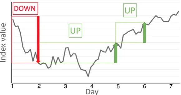
Fig. 3 shows the several types of windows to better understand the principle of how we determined direction of price change for the time windows. In this example, the maximal window size is 3 days and threshold value are 7 units for the “down” window and 3 units for the “up” window. The window marked “down” represents a sudden fall of price within one day. The following “up” window is an example of a slow, gradual change of price with a local maximum on day 3, local minimum on day 4 and finally a threshold value on day 5. The last window indicates a rapidly growing trend which reaches a threshold value within one day.
Classification
We used text classification to predict whether the given document is connected with an upward or downward movement of the S & P 500 Index. Based on its publication date, each document was connected to a corresponding time window (found in previous step) and assigned a class (1 for downward and 2 for upward movement). The documents collection was processed for all 9 sets of time windows and 9 classification sets were created.
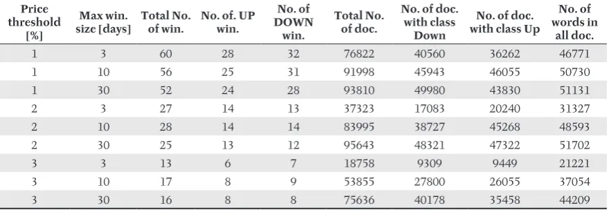
Tab. I shows the basic statistics of used data sets used for classification. We can see that the number of text documents was in a range of 3732395643, document collection contained 21221‑51702
words and that data sets are well balanced between the two classes.
Text pre‑processing and conversion
The raw text of each document was processed as follows:
1) Remove all whitespace. 2) Lowercase all letters.
3) Tokenize the document – get words (using TreebankWordTokenizer).
4) Filter words – the minimal word length was three letters and all numbers were excluded.
The edited text was converted into a structured format by using a Python library scikit‑learn and its Vectorizer class. Only words that occurred at least 10 times in the whole document collection were included in the resulting vector representation, because this minimal number of occurrences provides the best results and speeds up processing time.
The documents were converted to the bag‑of‑words representation using TF‑IDF (local weight multiplied by global weight) weighting scheme for the term‑document matrix (Weiss, 2010). The reason for this was that this scheme provided in previous experiments the best results.
Training and testing
The converted data was split into the training (60 %) and testing (40 %) set (this ratio was chosen to not overfit the classifier and properly test the created model on unknown data). Each bag‑of‑words representation was processed by 6 classifiers (with default settings – no parameter optimization was made) in scikit‑learn. The classifier’s performance was evaluated by the achieved accuracy (proportion of the correctly classified instances on all examined instances on the test set (Go, 2009)).
The following classification algorithms were used: • Multinomial Naive Bayes
• Bernoulli Naive Bayes • Logistic Regression • Decision Tree Classifier • Random Forest Classifier • Linear SVC
I: Basic statistics of data sets used for classification
Price threshold [%] Max win. size [days] Total No. of win.
No. of. UP win. No. of DOWN win. Total No. of doc.
No. of doc. with class
Down
No. of doc. with class Up
No. of words in
all doc.
1 3 60 28 32 76822 40560 36262 46771
1 10 56 25 31 91998 45943 46055 50730
1 30 52 24 28 93810 49980 43830 51131
2 3 27 14 13 37323 17083 20240 31327
2 10 28 14 14 83995 38727 45268 48593
2 30 25 13 12 95643 48321 47322 51702
3 3 13 6 7 18758 9309 9449 21221
3 10 17 8 9 53855 27800 26055 37054
They were used because they are available in scikit‑learn, represent different types of classification algorithms and provided good results in previous experiments of the authors.
RESULTS
One set of text data (Yahoo articles) together with 9 sets of S & P 500 Index values divided into time windows were used to prepare the data for the classification. The class‑labelled data sets were processed using TF‑IDF weighting scheme by 6 classification algorithms. In total, 9 classification results were obtained.
Tab. II shows classification results for 9 different data sets based on generated time windows. We can see that the accuracy is in range from 65 % to 74 %. Regarding classification algorithms, the best accuracy provided decision trees and Linear SVC. If we compare the results to other works mentioned in the Literature overview, we can see that the achieved accuracy is lower (Bollen, 2011 achieved about 90 %). However, our method focused on longer time intervals than only one day. We showed that it is, with a rather high accuracy, possible to determine if the document is part of downward or upward price movement.
II: Best classification result for each data set
Price threshold [%]
Max win.
size [days] Best classifier accuracy precision recall F1 score
1 3 Decision Tree 0.6531 0.6531 0.6531 0.6531
1 10 Random Forest 0.6714 0.6755 0.6714 0.6691
1 30 Decision Tree 0.6815 0.6815 0.6815 0.6815
2 3 LinearSVC 0.6753 0.6742 0.6753 0.6743
2 10 Decision Tree 0.6913 0.6913 0.6913 0.6913
2 30 Decision Tree 0.6825 0.6825 0.6825 0.6825
3 3 Linear SVC 0.6903 0.6903 0.6903 0.6903
3 10 Decision Tree 0.7093 0.7094 0.7093 0.7093
3 30 Linear SVC 0.7415 0.7412 0.7415 0.7412
CONCLUSION
The goal of the work was to examine whether the content of text documents published on the Internet (specifically Yahoo news articles posts) has any connection with stock price movements. We used the values of the S & P 500 Index and divided them into time windows with either growing or decreasing index value trend. Subsequently, we examined (using the classification accuracy) the connection between the documents’ content and the trend of the index value in the time window in which was the document published.
The achieved accuracy around 70 % tells us that the news articles which are published about companies are partially related to the performance of the whole stock index. Of course, there is the chicken or the egg causality dilemma – do the news articles influence the stock price changes or are they just a reaction to the changes? The used methodology was based on the premise that based on the document’s text we can predict whether the document is part of a downward or upward price movement. This means that document could be published at the very start of the movement and therefore could influence future price. However, it could be also published in the middle or the end of the movement and therefore be in fact a reaction to the past changes. Our results indicate there is indeed a causal relation between texts and prices, but we give no definitive answer about the direction of this relation.
Regarding used classification algorithms, it was discovered that the best results provided decision tree classifiers and Linear SVC. It must be noted that we did not optimize the parameters of used classification algorithms. By doing this, we might achieve a slightly higher accuracy.
This area could be further researched in various directions. Firstly, the analysis may be performed on more types of documents (e.g., newspaper articles). Secondly, the class assigning method may be enriched by using various thresholds of the index value changes (not only 5 %). Thirdly, it might be interesting to examine not the whole stock index, but the stock prices of the individual companies instead.
Acknowledgement
“Knowledge mining in continuous textual sources with a changing concept”] and Internal Grant Agency of Mendel University [No. PEF_DP_2018016 “Text analysis by machine learning with a focus on the stock market”].
REFERENCES
AGGARWAL, C. C. 2007. Data Streams: Models and Algorithms. Springer.
BOLLEN, J., MAO, H. and ZENG, X. 2011. Twitter mood predicts the stock market. Journal of Computational Science, 2(1): 1–8.
CHANG, P. C. and LIU, C. H. 2008. A TSK type fuzzy rule based system for stock price prediction. Expert Systems with applications, 34(1): 135–144.
DARENA F., PETROVSKY J., ZIZKA, J. and PRICHYSTAL, J. 2018. Machine Learning‑Based Analysis of the Association between Online Texts and Stock Price Movements. Inteligencia Artificial, 21(61): 95–110. DENG, S., MITSUBUCHI, T., SHIODA, K., SHIMADA, T. and SAKURAI, A. 2011. December. Combining
technical analysis with sentiment analysis for stock price prediction. In: 2011 IEEE Ninth International Conference on Dependable, Autonomic and Secure Computing. IEEE, pp. 800–807.
DI PERSIO, L. and HONCHAR, O. 2016. Artificial Neural Networks architectures for stock price prediction: comparisons and applications. International Journal of Circuits, Systems and Signal Processing, 10: 403–413. FALINOUSS, P. 2007. Stock Trend Prediction Using News Articles A Text Mining Approach. Tarbiat Modares
University.
GAMA, J. 2010. Knowledge discovery from data streams. CRC Press.
GIOT, P. 2005. Market risk models for intraday data. The European Journal of Finance, 11(4): 309–324.
GO, A., BHAYANI, R. and HUANG, L. 2009. Twitter sentiment classification using distant supervision. CS224N Project Report. Stanford.
GROTH, S. S. and MUNTERMANN, J. 2011. An intraday market risk management approach based on textual analysis. Decision Support Systems, 50(4):680–691.
GUHA, S., KIM, C., SHIM, K. GUHA, S., KIM, C. and SHIM, K. 2004. XWAVE: optimal and approximate extended wavelets. In: Proceedings of the thirtieth international conference on very large data bases. Vol 30. Toronto, Canada, August 31 ‑ September 03, 2004, pp. 288–299.
HAFEZI, R., SHAHRABI, J. and HADAVANDI, E., 2015. A bat‑neural network multi‑agent system (BNNMAS) for stock price prediction: Case study of DAX stock price. Applied Soft Computing, 29: 196–210.
HAGENAU, M., LIEBMANN, M. and NEUMANN, D., 2013. Automated news reading: Stock price prediction based on financial news using context‑capturing features. Decision Support Systems, 55(3): 685–697.
HAN, J., KAMBER, M. and PEI, J. 2012. Data Mining: Concepts and Techniques. 3rd Edition. Waltham,
MA: Morgan Kaufmann.
HO, R. 2010. Map Reduce and Stream Processing. Pragmatic Programming Techniques. [Online]. Available at: http://horicky.blogspot.cz/2010/11/map‑reduce‑and‑stream‑processing.html [Accessed: 2018, October 17]. HULTEN, G., SPENCER, L., and DOMINGOS, P. 2001. Mining time‑changing data streams. In: ACM
SIGKDD Intl. Conf. on Knowledge Discovery and Data Mining. New York: AMC, pp. 97–106.
KARGUPTA, H., PARK, B. H., PITTIE, S., LIU, L., KUSHRAJ, D., and SARKAR, K. 2002. MobiMine: Monitoring the Stock Market from a PDA. ACM SIGKDD Explorations, 3(2): 37–46.
KEARNEY C. and LIU, S. 2014. Textual sentiment in finance: A survey of methods and models. International Review of Financial Analysis, 33: 171–185.
KOGAN, S., LEVIN, D., ROUTLEDGE, B. R., SAGI, J. S. and SMITH, N. A. 2009. Predicting risk from financial reports with regression. In: Proceedings of Human Language Technologies: The 2009 Annual Conference of the North American Chapter of the Association for Computational Linguistics. Association for Computational Linguistics, pp. 272–280.
LEE, H., SURDEANU, M., MACCARTNEY, B. and JURAFSKY, D. 2014. On the Importance of Text Analysis for Stock Price Prediction. In: Proceedings of the 9th International Conference on Language Resources and Evaluation, LREC 2014. European Language Resources Association, pp. 1170–1175.
LIN, X., YANG, Z. and SONG, Y. 2009. Short‑term stock price prediction based on echo state networks. Expert systems with applications, 36(3): 7313–7317.
LO, A. W. 2001. Risk management for hedge funds: introduction and overview. Financial Analysts Journal, 57(6): 16–33.
MANYIKA, J., CHUI, M., BROWN, B., BUGHIN, J., DOBBS, R., ROXBURGH, C., and BYERS, A. H. 2011. Big Data: The Next Frontier for Innovation, Competition, and Productivity. Report. McKinsey Global Institute. MITTERMAYER, M. A. 2004. Forecasting intraday stock price trends with text mining techniques. In: HICSS
‘04 Proceedings of the Proceedings of the 37th Annual Hawaii International Conference on System Sciences (HICSS’04).
Volume 3. Washington, DC: IEEE.
NETOLICKÝ, P., PETROVSKÝ, J., DAŘENA, F. and ŽIŽKA, J. 2017. Text Classification Using Time Windows Applied to Stock Exchange. International Journal of New Computer Architectures and their Applications, 7(2): 62–67.
SCHUMAKER, R. P. and CHEN, H., 2009. Textual analysis of stock market prediction using breaking financial news: The AZFin text system. ACM Transactions on Information Systems, 27(2): 12.
WANG, B., HUANG, H. and WANG, X., 2012. A novel text mining approach to financial time series forecasting. Neurocomputing, 83: 136–145.
WANG, Y. 2017. Stock market forecasting with financial micro‑blog based on sentiment and time series analysis. Journal of Shanghai Jiaotong University (Science), 22(2): 173–179.
WEISS, S. M., INDURKHYA, N. and ZHANG, T. 2010. Fundamentals of Predictive Text Mining. London: Springer. WUTHRICH, B., CHO, V., LEUNG, S., PERMUNETILLEKE, D., SANKARAN, K. and ZHANG, J. 1998. Daily stock market forecast from textual web data. In: SMC’98 Conference Proceedings. 1998 IEEE International Conference on Systems, Man, and Cybernetics. Cat. No. 98CH36218. Vol. 3. IEEE, pp. 2720–2725.
Contact information Pavel Netolický: [email protected]