SEPARATING NONLINEAR IMAGE MIXTURES USING A PHYSICAL MODEL TRAINED
WITH ICA
Mariana S. C. Almeida and Lu´ıs B. Almeida
Instituto de Telecomunicac¸˜oes
Instituto Superior T´ecnico
Av. Rovisco Pais – 1, 1049-001 Lisboa, Portugal
[email protected], [email protected]
ABSTRACT
This work addresses the separation of real-life nonlinear mixtures of images, which occur when a paper document is scanned and the image from the back page shows through. A physical model of the mixing process, based on the con-sideration of the halftoning process used to print grayscale images, is presented. The corresponding inverse model is then used to perform image separation. The parameters of the inverse model are optimized through the MISEP tech-nique of nonlinear ICA, which uses an independence crite-rion based on minimal mutual information.
The quality of the separated images is competitive with the one achieved by other techniques, namely by MISEP with a generic MLP-based separation network and by De-noising Source Separation. The separation results show that MISEP is an appropriate technique for training the para-meters and that the model fits the mixing process well, al-though not perfectly. Prospects for improvement of the model are presented.
1. INTRODUCTION
When scanning or photographing a paper document, inter-ference of the back page image on the front page one is a common problem, especially if the paper is thin or rather transparent. In this paper we focus on a difficult version of this problem, in which the paper is of the onion skin type, which creates a strong, significantly nonlinear mix-ture. The mixtures that we use were obtained by printing images and/or text on both sides of a sheet of onion skin, which was then scanned, on both sides, with a desktop scan-ner. The scanned images of each pair were then aligned with each other. The source images were also aligned with the mixture ones, for quality assessment. A more complete description of the image preparation procedure is given in [1].
This work was partially supported by FCT project POSC/EEA-CPS/61271/2004.
These images have already been used to test other sepa-ration methods, mentioned ahead, and are available athttp: //www.lx.it.pt/∼lbalmeida/ica/seethrough/ index.html. Due to lack of space, we only show the first pair of source and mixture images (Fig. 3). The other four pairs can be found in [1] and in the mentioned web location. Reconstructing two sources from two mixtures can be seen as a blind source separation (BSS) problem. BSS is often achieved by assuming that the sources are statistically independent from each other and performing independent component analysis (ICA). Linear ICA is a well studied problem with essential uniqueness of the solution [2]. Non-linear ICA is still much less studied. With no additional constraints it is an ill-posed problem, having an infinite num-ber of solutions that are not related to one another in any simple way [3] [4] .
The problem under study is especially challenging be-cause it involves a real-life nonlinear, noisy mixture and, furthermore, some pairs of source images do not satisfy the independence assumption. Due to the small number of pa-rameters under estimation and to the simplicity of the map-ping, linear ICA often recovers the sources satisfactorily from linear mixtures, even if they are not completely inde-pendent. However, in nonlinear mixtures the quality of the separation can easily be impaired when the independence assumption is not met [1].
In this paper we first present a physical model of the mixture process. Then, the inverse of that model is used to perform separation. The parameters of the inverse model are estimated through an ICA criterion, using the MISEP method [5]. The results show that a separation with a good quality is achieved. The small number of degrees of free-dom of the model eliminates the ill-posedness that is nor-mally associated with less constrained nonlinear ICA.
the MISEP method of nonlinear ICA with a multilayer per-ceptron as separating system and with regularization con-straints to deal with the ill-posedness of nonlinear ICA [1]. The other approach was the use of the nonlinear denoising source separation (DSS) method [6], which is not based on an independence criterion, but instead uses some basic prior knowledge about images to perform separation. The sepa-ration results presented in this paper are competitive with those obtained with those methods, as evidenced by objec-tive quality measures that we include ahead.
The same separation problem is also addressed in an-other paper in this conference [?]1. That paper presents a
non-iterative separation method, based on the sparsity of the coefficients of the wavelet decomposition of images.
This manuscript is organized as follows: Section II briefly describes the MISEP method. Section III describes the mix-ing model and its inverse. Section IV presents experimen-tal results, including objective quality measures. Section V concludes and presents future research directions.
2. OVERVIEW OF THE MISEP METHOD
MISEP is a generalization of the well known INFOMAX technique of linear ICA [7]. INFOMAX maximizes the en-tropy of the output of the network depicted in Fig. 1. Block F performs the linear separation. The separated compo-nents areyi. Blocksψiare auxiliary, being used only dur-ing the traindur-ing phase. Each of these blocks implements an invertible, increasing transformationzi=ψi(yi), whose co-domain is the interval[0,1]. Ideally each of these blocks should implement the cumulative distribution function (cdf) of the corresponding inputyi. In that case, maximizing the output entropy corresponds to minimizing the mutual infor-mation (MI) between the extracted componentsyi. Thus, INFOMAX performs linear ICA by indirectly minimizing the mutual information of the sources. Due to the small number of parameters under estimation, linear separation can often be achieved by INFOMAX even if theψi blocks implement only crude approximations of the cdfs of the sources. In nonlinear ICA, however, the correct estimation of the cdfs plays a more crucial rule.
MISEP extends INFOMAX in two directions. First, MISEP handles nonlinear mixtures, by allowing block F to be nonlinear. Second, MISEP uses output nonlinearities that adapt to the statistical distributions of the extracted compo-nents. In MISEP, the maximization of the entropy of the output of the network of Fig. 1 simultaneously optimizes theψifunctions and the separation mapping.
MISEP can use any parameterized, linear or nonlinear block in F. In previous tests with the present dataset [1], this block was implemented by means of a multilayer per-ceptron with suitable regularization. In this paper, block F
1To be added in the final version if the other paper is accepted.
Fig. 1. Network structure used in INFOMAX and in MISEP. In INFOMAX, F is an adaptive linear block and theψiare fixed a priori. In MISEP, F can be nonlinear and both F and ψiare adaptive.
will consist of the inverse of the mixture model, to be pre-sented in the next section. For more details on MISEP see [5, 1].
3. MIXING MODEL
The physical mixture model that we use was originally de-veloped by Miguel Faria and Luis B. Almeida [8], but its parameters had only been manually adjusted, having never been estimated in a form similar to the one presented in this paper. We present the model in some detail here because it had not been previously described in any widely available publication.2
The model takes into account that the printer produces only black dots, using a halftoning process to produce gray tones. Halftoning consists of using a very large number of tiny black dots, whose intensities are averaged out by our eyes, giving the appearance of gray. The level of gray de-pends on the fraction of area covered by black dots. With the low scanning resolution that was used in the dataset (100 dpi), each scanned pixel encompasses a large number of halftoning dots, and therefore the pixel’s intensity also de-pends on the fraction of area covered by the dots.
We represent the actual printed intensity at a given point in the page bysˆ. Since the printer only produces black and white,sˆ ∈ {0,1}, with 0 representing black and 1 repre-senting white. The halftoning process is modeled by con-sideringsˆto be a random variable which takes independent values in different locations of the image, with a distribu-tion defined by the probabilityP(ˆs= 1). This probability is equal, at each point, to the intensity of the image being printed (the source image). The mean intensity at a given point is given by the expected value
s=E(ˆs) =P(ˆs= 1) (1)
at that point. We denote it byssince it corresponds to the intensity of the source image. Labeling the two sides of
2An equivalent model was developed by Stefan Harmeling without any
the paper with subscripts 1 and 2 respectively, we have the following relationships for the two sources:
s1 = P(ˆs1= 1)
s2 = P(ˆs2= 1). (2)
With a semi-transparent paper like onion skin, the ob-served intensity on each side of the paper depends on what is printed on both sides. Assume that we are observing the document from side number 1. The observed intensity at each point can take only four levels:
ˆ xi =
⎧ ⎪ ⎪ ⎨ ⎪ ⎪ ⎩
l1 if ˆs1= 0 and ˆs2= 0 l2 if ˆs1= 0 and ˆs2= 1 l3 if ˆs1= 1 and ˆs2= 0 l4 if ˆs1= 1 and ˆs2= 1
(3)
The values ofl1,· · ·, l4 depend on the physical properties of the paper and of the scanner, and also on the printing process. Due to physical constraints, we know thatl1 ≤ l2 ≤l3 ≤l4, with strict inequality holding if the paper is not completely opaque and not completely transparent.
The mean intensity at each point, observing from side 1 of the paper, is given by the expected value
x1 = E(ˆx1)
= l1P(ˆs1= 0,s2ˆ = 0) +l2P(ˆs1= 0,ˆs2= 1) + l3P(ˆs1= 1,s2ˆ = 0) +l4P(ˆs1= 1,ˆs2= 1).
This is what corresponds, in our model, to the intensity ac-quired by the scanner.
We shall assume that ˆs1 ands2ˆ are independent from each other. Taking (2) into account,
x1=l1(1−s1)(1−s2)+l2(1−s1)s2+l3s1(1−s2)+l4s1s2. (4) Assuming that the printing and acquisition systems are sym-metrical, i.e., that they treat both sides of the paper in the same way, we have
x2=l1(1−s1)(1−s2)+l2s1(1−s2)+l3(1−s1)s2+l4s1s2. (5) In order to simplify these equations we can define the fol-lowing parameters:
α=l3−l1 β=l2−l1
γ=l4+l1−l2−l3 δ=l1
(6)
Substituting into (4) and (5) we get the following equations
x1 = αs1+βs2+γs1s2+δ (7) x2 = αs2+βs1+γs1s2+δ, (8)
This shows that the mixture is bi-affine (it is affine as a function of each of the sources, if the other source is kept constant). The parameters of the mixture (α, β, γ, δ) have a direct correspondence with the intensity levels li of the four possible combinations that result from the halftoning process. If the paper is not perfectly transparent,l3 = l2 and consequentlyα=β, which is required for the model to be invertible.
To recover the sources from the mixtures, we must now invert the model (7, 8). Subtracting (7) from (8) we see that s1ands2are related by
s2=s1+ (x2−x1)/(α−β). (9)
Substituting now (9) into (7) we get a quadratic equa-tion,
γs2 1+
α+β+γ(x2α−−βx1)
s1−x2+δ+α(x2α−−βx1)= 0 (10) which can be explicitly solved. We first define
a=γ
b=α+β+γ(x2−x1)
α−β
c=−x2+δ+α(xα2−−βx1).
(11)
Sources1is then given by
s1= −b+
√
b2−4ac
2a . (12)
One can check that using a minus sign before the square root, in the latter expression, would not yield a solution of (7, 8). Only the plus sign yields a valid solution.
It would be possible to find an equation similar to (12) fors1. However, once we have computeds1, we can use (9) to calculates2. This simplifies the calculation of both s2and its derivatives, which are needed in MISEP. The use of the intermediate variables a,b andc not only helps to invert the system but also greatly simplifies the computation of the derivatives that are required in MISEP, allowing a significant increase in optimization speed.
The model that we have described doesn’t take into ac-count any lateral diffusion of light in the onion skin paper. At the low scanning resolution that was used this seems to be a reasonable approximation, as evidenced by the results presented ahead.
4. EXPERIMENTS
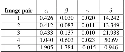
Image pair α β γ δ 1 0.426 0.030 0.020 14.242 2 0.412 0.083 0.011 13.349 3 0.433 0.137 0.010 21.938 4 1.040 0.603 0.023 50.69 5 1.905 1.784 -0.015 0.946
Table 1. Parameters obtained after training the model using, as training set, each of the five pairs of mixtures.
close to the identity function (α= 1,β= 0.01,γ= 0.001, δ= 0.001).
For each pair of mixture images, 1000 pairs of pixels were randomly chosen as training set. One separation model was trained, during 1000 epochs, for each pair of images, leading to the parameter values shown in Table 1.3 It is
in-teresting to note that the estimated parameters differ some-what among the various pairs of images, although the print-ing and acquisition was performed in as similar a manner as possible for all images, leading one to expect that the same model would fit all mixtures.
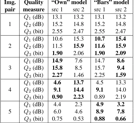
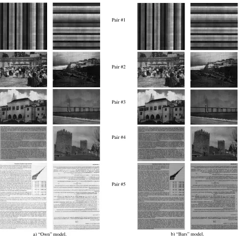
Each mixture was separated using the model trained for that mixture (which we call the mixture’s “own model”). The results are shown in the left half of Fig. 4. The model trained for the “bars” images can, in some sense, be consid-ered to be the most basic and most “universal” one, because in that case the source images are independent from each other by construction, and have almost uniform intensity distributions. For that reason we also tried using that model (which we call the “bars” model) to separate the other four mixtures. The results are shown in the right half of Fig. 4. The results obtained with the two models are similar in all cases except for the last image pair, which corresponds to a mixture of images containing mostly text. This is also the pair for which the estimated parameters differ most from those of the “bars” images (see Table 1).
The scatter plots of the sources, mixture components and separated components, for the “bars” pair, are shown in Fig. 2. We can see that the model achieved a good, but not perfect separation. The fact that the scatter plot of the separated components shows curved boundaries is probably due to some imperfection of the model. We discuss this fur-ther in the Conclusions.
4.1. Quality measures
To analyze the quality of the separated images in a more objective way we computed three quality measures that had already been used for the same mixing problem in [1], [6].
3In the tests, the range of image intensity values that was used was [0,255], instead of the range[0,1]used in the derivations of Section 3. The parameter values shown in the table correspond to the range[0,255].
a) Sources b) Mixtures c) Separated components
Fig. 2. Scatter plots corresponding to the “bars” pair.
The first quality measure,Q1, is simply the signal to noise ratio (SNR) between each extracted component and the cor-responding source. The second quality measure, Q2, is the signal to noise ratio, compensated for possible nonlin-ear transformations of the intensity scales of the estimated sources. The third measure,Q3, is the mutual information between each extracted component and the corresponding source. The mutual information was estimated, in each case, from a set of 5000 randomly selected pixel pairs, chosen in-dependently from those forming the training set, and was computed using the I(1) estimator described in [9], with k = 3. More details about these measures can be found in [1]. We didn’t use measureQ4, from that reference, because it had shown, in previous tests, not to be a reliable measure of separation quality [1, 6].
Table 2 contains the values of the quality measures of the components obtained, for each pair, with the “own” model and with the “bars” model. Table 3 shows the results ob-tained with the “own” model, together with results obob-tained with MISEP using an MLP as a separator [1], and with re-sults obtained with nonlinear DSS [6]. The table also shows, for comparison, in column MSE, the quality values of what could be considered an “ideal” separation: the result ob-tained by training an MLP with the two mixture pixels as inputs and with the two source pixels as desired outputs. The results for the fourth and fifth image pairs are not shown in the table because they were not available for both of the other separation methods. The model proposed in this paper performed better, on average, than both MLP-based MISEP and nonlinear DSS.
5. CONCLUSIONS
The inverse of a physical model of the mixture process was used to perform the separation of a nonlinear real-life mix-ture of images. The model’s parameters were estimated by the MISEP method, which uses an ICA criterion.
The separation results are competitive with those ob-tained with other methods, namely with MLP-based MISEP and with nonlinear DSS. They show, on the one hand, that the mixture model is appropriate for the problem being ad-dressed and, on the other hand, that MISEP is an adequate technique for estimating the model’s parameters.
Img. Quality “Own” model “Bars” model pair measure src 1 src 2 src 1 src 2
Q1(dB) 13.1 13.2 13.1 13.2 1 Q2(dB) 15.2 14.8 15.2 14.8 Q3(bit) 2.55 2.47 2.55 2.47 Q1(dB) 10.6 15.3 10.7 15.4 2 Q2(dB) 11.5 15.9 11.6 15.9 Q3(bit) 1.90 2.06 1.90 2.09 Q1(dB) 14.9 7.6 14.7 8.6 3 Q2(dB) 15.8 8.5 15.7 9.4 Q3(bit) 2.27 1.46 2.25 1.59 Q1(dB) 4.6 13.7 4.5 13.3 4 Q2(dB) 9.1 14.4 9.1 14.0 Q3(bit) 0.90 2.23 0.89 2.19 Q1(dB) 4.4 2.3 4.9 3.2 5 Q2(dB) 6.0 4.6 8.9 7.8 Q3(bit) 0.75 0.53 0.88 0.66
Table 2. Values of the quality measures for the results ob-tained with the “own” model and with the“bars” model. The best results are shown in bold.
possible cause could be the existence of gamma correction in the scanning process, which was not accounted for in the model, and which would produce a nonlinear distortion of the gray scales of the mixture images. This could explain the curvature observed in the boundaries of the scatter plot of the separated components. Incorporating gamma correc-tion in the model will involve the addicorrec-tion of just one more parameter and may lead to a more perfect separation.
Another planned improvement involves the explicit in-corporation of noise in the model. Noise is clearly present in the mixture process, as evidenced by the scatter plots that were presented. The strongest source of noise probably is the inhomogeneity of the paper. The incorporation of noise in the model may lead to a better estimation of the source images.
A more complex improvement will consist of taking into account the non-local character of the mixture. This will become important as the scanning resolution is increased above the one used in this work.
6. REFERENCES
[1] L.B. Almeida, “Separating a real-life nonlinear image mixture,” Journal of Machine Learning Research, vol. 6, pp. 1199–1229, July 2005.
[2] P. Comon, “Independent component analysis – a new concept?,” Signal Processing, vol. 36, pp. 287–314, 1994.
[3] A. Hyv¨arinen and P. Pajunen, “Nonlinear independent
Img. Quality “Own” MISEP Nonl. MSE
pair measure model MLP DSS
Q1(dB) 13.2 13.5 14.4 14.9 1 Q2(dB) 15.0 14.5 15.0 15.3 Q3(bit) 2.51 2.42 2.54 2.55 Q1(dB) 13.0 11.6 10.0 13.4 2 Q2(dB) 13.7 13.0 12.3 13.8 Q3(bit) 1.98 1.89 1.77 2.00 Q1(dB) 11.2 10.3 11.4 12.5 3 Q2(dB) 12.1 11.6 12.7 13.1 Q3(bit) 1.87 1.74 1.93 1.95 Q1(dB) 12.4 11.8 11.9 13.6 Mean Q2(dB) 13.6 13.0 13.3 14.1 Q3(bit) 2.12 1.98 2.07 2.18
Table 3. Values of the quality measures, averaged across all image pairs, for three separation methods. The best results are shown in bold. For comparison, column MSE shows the quality of what could be considered an “ideal” separation.
component analysis: Existence and uniqueness results,”
Neural Networks, vol. 12, no. 3, pp. 429–439, 1999.
[4] G.C. Marques and L.B. Almeida, “Separation of non-linear mixtures using pattern repulsion,” in Proc. First
Int. Worksh. Independent Component Analysis and Sig-nal Separation, J. F. Cardoso, C. Jutten, and P.
Louba-ton, Eds., Aussois, France, 1999, pp. 277–282.
[5] L.B. Almeida, “MISEP – Linear and nonlinear ICA based on mutual information,” Journal of Machine Learning Research, vol. 4, pp. 1297–1318, 2003.
[6] M. S.C. Almeida, H. Valpola, and J. S¨arel¨a, “Separa-tion of nonlinear image mixtures by denoising source separation,” in Proc. Int. Worksh. Independent
Compo-nent Analysis and Blind Source Separation, Charleston,
South Carolina, U.S.A., 2006, Lecture Notes in Artifi-cial Intelligence, pp. 8–15, Springer-Verlag.
[7] A. Bell and T. Sejnowski, “An information-maximization approach to blind separation and blind deconvolution,” Neural Computation, vol. 7, pp. 1129– 1159, 1995.
[8] L.B. Almeida and M. Faria, “Separating a real-life non-linear mixture of images,” in Proc. Int. Worksh.
Inde-pendent Component Analysis and Blind Source Separa-tion, Carlos G. Puntonet and Alberto Prieto, Eds. 2004,
number 3195 in Lecture Notes in Artificial Intelligence, pp. 729–736, Springer-Verlag.
a) Sources. a) Mixtures.
Fig. 3. Sources and mixtures of the first pair of images.
a) “Own” model.
Pair #1
Pair #2
Pair #3
Pair #4
Pair #5
b) “Bars” model.